Technology and Investment
Vol.3 No.2(2012), Article ID:19397,5 pages DOI:10.4236/ti.2012.32015
Pricing Callable Bonds Based on Monte Carlo Simulation Techniques
1Faculty of Science and Technology, University of Macau, Macao, China
2Faculty of Business Administration, University of Macau, Macao, China
Email: {dding, jackyso}@umac.mo, *umacfuqi@gmail.com
Received March 20, 2012; revised April 23, 2012; accepted April 30, 2012
Keywords: Callable Bond; Monte Carlo Simulation; CIR Model; Embedded Option Pricing
ABSTRACT
In this paper, a Monte Carlo method, which is based on some new simulation techniques proposed recently, is presented to numerically price the callable bond with several call dates and notice under the Cox-Ingersoll-Ross (CIR) interest rate model. The corresponding algorithms are also presented to practical callable bond pricing. The numerical experiments show that this method works very well for callable bond under the CIR interest rate model.
1. Introduction
A callable bond is a bond that allows the issuer to buy back the bonds from the bond holders at pre-specified prices on the pre-specified call dates. Therefore, a callable bond is a straight bond embedded with a call of European option (a single call date) or Bermudan option (several call dates). However, this option is an integral part of a bond, and cannot be traded alone, and hence, its prices cannot be observed. Thus, the callable bond pricing must be involved in the pricing problem of the corresponding option.
There are some different approaches for pricing callable bonds. The first approach is based on the BlackDerman-Toy model, which was presented in [1] (2006), with the discrete simulation of binary tree. With the help of the risk-neutral valuation, the second approach is to obtain a partial differential equation (PDE) subject to appropriate boundary conditions based on the equilibrium interest rate model. Since it is very difficult to analytically solve this PDE, some different discretizations and different numerical methods have been proposed. Büttler in [2] (1995) applied finite difference method to find the evaluation of callable bonds. Büttler and Waldvogel in [3] (1996) derived an analytic expression for the Green's function of the corresponding PDE for certain specific interest rate models, and developed a semi-analytic method for pricing callable bonds with notice. As the further development, the finite volume method was used by D’Halluim et al. in [4] (2001), and the finite element method was considered by Farto and Vázquez in [5] (2005) for the numerically pricing callable bonds with notice. Recently, a dynamic programming approach was proposed by Ben-Ameur et al. in [6] (2007) for numerically pricing options embedded in bonds. In this dynamic programming approach they used finite difference method and solved the Green’s function by conditional distributions and expectations with piecewise-linear approximation.
Meanwhile, in the last decade, many new numerical schemes for simulations of interest rate models, especially, the Cox-Ingersoll-Ross (CIR) interest rate model, have been proposed. For instance, the balanced implicit method (BIM) was proposed by Milstein et al. in [7] (1998), the balanced Milstein method (BMM) was developed by Kahl and Schurz in [8] (2006). Also, the exact transition distribution method (ETD) is considered to simulate the square-root diffusions (e.g. see [9]). Recently, a new splitting-step scheme was presented by Ding and Chao in [10] (2009). In this paper, based on these new simulation techniques we present a Monte Carlo method to numerically price the Bermudan-type callable bond with notice.
This paper is structured as follows. After this introduction, the interest rate models are reviewed, and several numerical simulation techniques are surveyed in Section 2. Then, based on these simulation techniques, an efficient Monte Carlo method is presented to price the callable bond with several call dates and notice under the CIR interest rate model in Section 3. The corresponding algorithms are presented in this section. Finally, numerical experiments for a practical callable bond with 10 call dates and 2 months notice are provided in Section 4. The numerical results of these experiments are also presented in this section, as well as some useful conclusions.
2. Simulations of Interest Rate Models
Pricing financial derivatives depends on the description of the dynamic process of underlying assets. Since the underlying asset of callable bond is the interest rate, we focus on the mathematical models for the interest rate. These models can be divided as single factor models and multiple factor models by the number of status variables.
The first well-known single factor model was proposed by Vasicek in [11] (1977). In this model, the interest rate  is give by the stochastic differential equation (SDE):
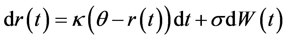 where
where ,
,  and
and  are all strictly positive constants, and
  is a standard Brownian motion. In detail,
  represents the speed at which
  reverts back to the long-term mean
 , while
  is the local volatility of short-term interest rates. The Ornstein-Uhlenbeck process is employed in this model for its key feature as the mean-reverting structure.
The Vasicek’s model has two significant failings. First, the interest rate can become negative; Second, empirical evidence suggests that the volatility of  is not constant as
 , but is an increasing function of
  instead. The first single factor model that possesses nonnegative interest rate is the CIR model, which was proposed by Cox, Ingersoll and Ross in [12] (1985). In this CIR model the interest rate
  follows the following SDE:
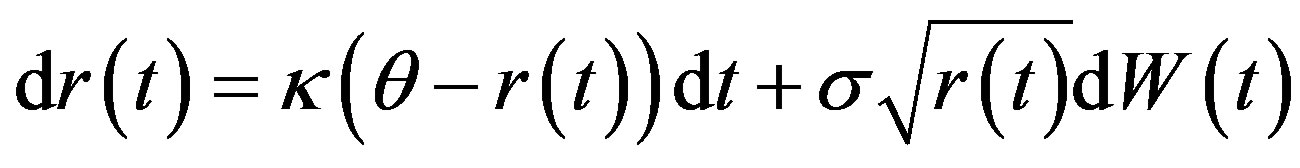 . (1)
. (1)
This model embodies the feature that the volatility is an increasing function of . In this paper we focus on this model.
Although the application of the Yamada’s condition reveals that the SDE (1) has a unique non-negative solution  for any given initial value
 , it is difficult to find an explicit formula for this solution. Thus, many practical applications lead to the numerical simulation of the CIR model. However, this involves two problems: The first one is that the numerical simulation would yield negative value in the general discretization of SDE (1); The second one is that, since the diffusion coefficient is not globally Lipschizian, the convergence of the general discretization for SDE (1) is not guaranteed.
In the last decade, many efficient new numerical schemes have been proposed for the CIR model (1) with positivity preservation. In the following, we survey these schemes, which are employed in the numerical experiments in Section 4.
Let  and let
  be a positive integer. In the following we denote
 , and set
  and
and  for each
 , i.e.
  is a partition of
 . We also denote
  for each
 . We assume that
  are
are  independent random variables having a common standard normal distribution.
The balanced implicit method (BIM) was proposed by Milstein et al. in [7]. The discretisation of the CIR model (1) by the BIM is given by
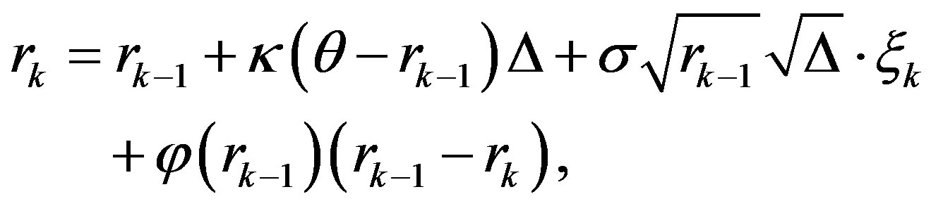 (2)
(2)
for each , where
  is called the control function, and here it is given by
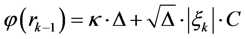 (3)
(3)
with  for
for ; and
; and  elsewhere. Here
  is selected as small as possible but halting the computation.
The balanced Milstein method (BMM) was developed by Kahl and Schurz in [8]. For CIR model (1) the BMM scheme is given by
 (4)
(4)
for each . BIM and BMM schemes preserve positivity for the CIR model (1) as
  tends to zero.
In the book [9], an algorithm for simulation of the CIR model (1) by the exact transition distribution (ETD) method is given in the following.
The CIR model (1) with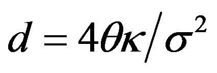 :
:
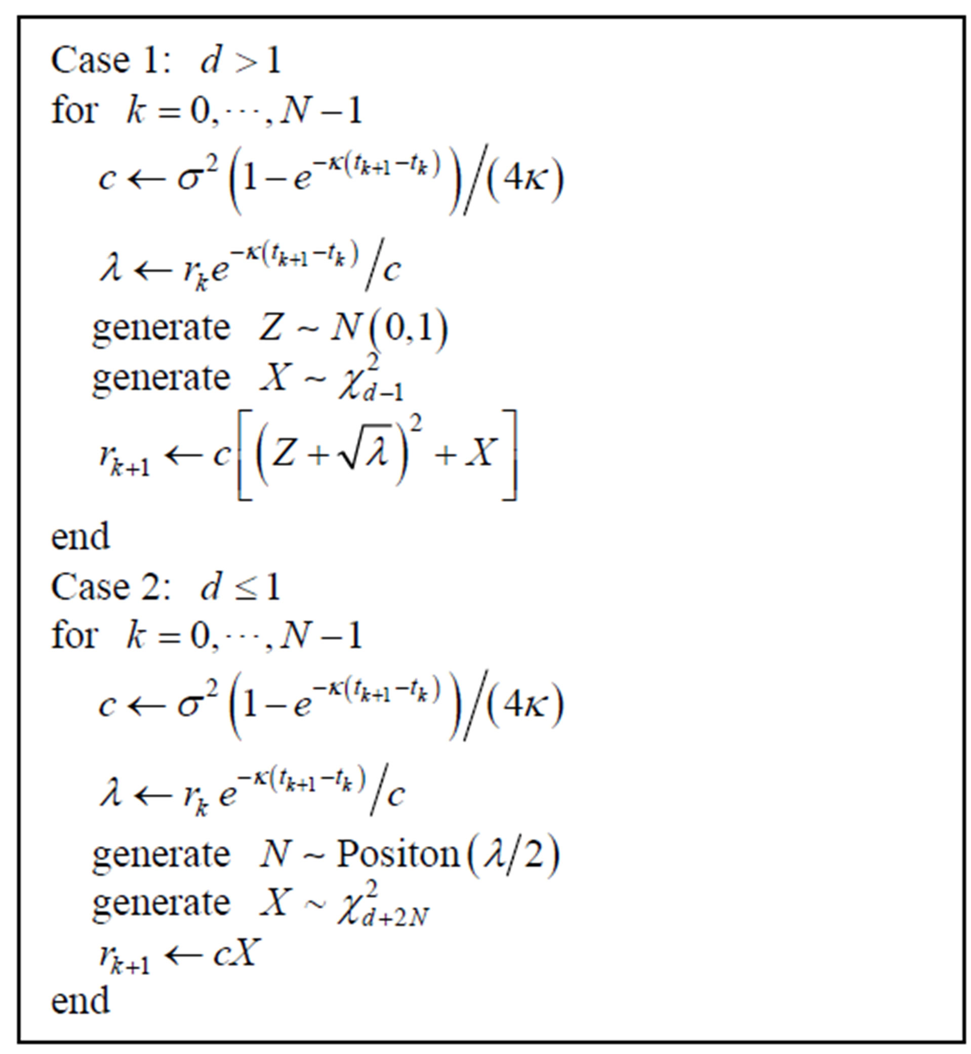
The advantage of this algorithm is the strict positivity preservation, comparing the conditional preservations of the two methods above. However, the ETD method suffers so great cost of computational time, and it also seems to be relatively unsuitable in our numerical experiments.
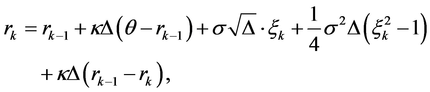
Recently, an efficient splitting-step scheme for the CIR model (1) was proposed by Ding and Chao in [10]. This new scheme, which is called the DC scheme here, is given as
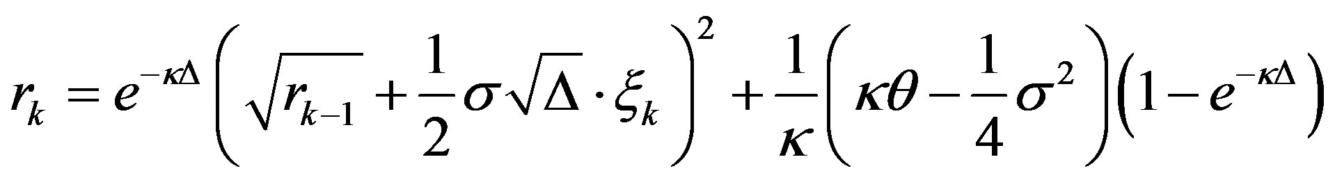 (5)
(5)
for each . This scheme preserves the positivity for the simulation in the case:
 , and it takes less computational time in comparison to BIM and BMM schemes.
3. The Monte Carlo Method
We consider a Bermudan callable bond which has  pre-specified coupon dates:
 where the bond may be redeemed at the last
  dates (call dates):
 . As in Figure 1, the notice period between each notice date and corresponding call date is denoted as
 . For convenience,
  is denoted the (n – j + 1)th notice date for each
  . In general, the time period between two coupon dates is one year, and the annual coupon payment is denoted as
 . At the call date
 , the call (or strike) price is defined as
 ,
, .
.
Let  and
and  denote the conditional expectation and conditional probability under the risk-neutral probability measure
 . For two dates
 , we define the discount factor over the time period
  when
when :
:
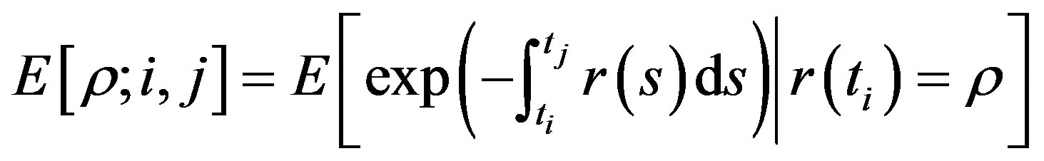 where
where  is the instantaneous interest rate with the initial value
 . For two notice dates
 , we also denote:
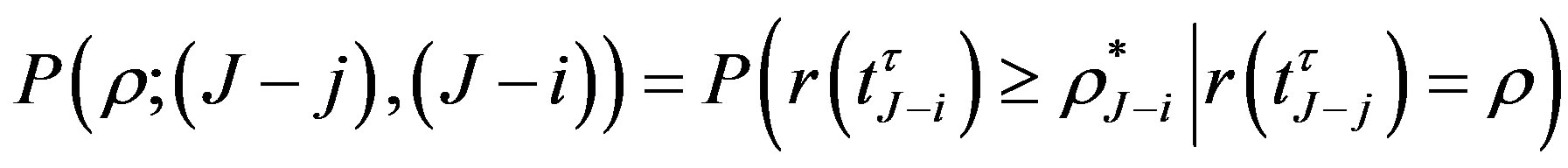 ,
,
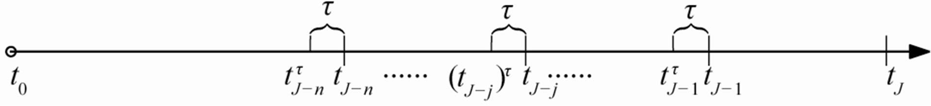
Figure 1. The call dates and the corresponding notice dates of Bermuda callable bond.
where  is the break-even (or critical) interest rate at the notice date
 . If the interest rate
  at the notice date
  is less than the break-even interest rate
  the issuer should call the bond at the call date
 , otherwise the debt (the callable bond in aspect of the issuer) should be hold.
Since the callable bond is embedded a Bermudan option, its value is computed recursively by the backward induction. At the first notice date , under the condition:
 , if the bond is not called, its value is given by
where  represents the date
 ; if the bond is called, the value is given by
 .
.
The issuer of the bond should minimizes his outstanding debt. If the price of the callable bond is greater than the time value of the call price including the coupon payment, he will call the bond to meet the requirement of the optimal call policy. That means he will choose the minimum value between uncall and call values, i.e., the value of the bond at the date  should be given by
To solve this optimal problem, we can consider the following equation for the variable :
:
 . (6)
. (6)
Then, the root of this equation is the break-even interest rate . There are some different methods to find this root. For the CIR model (1), the paper [3] gives a formula for the root:
 , (7)
, (7)
where , and functions
  and
and  are defined by
 ,
,  with
with  and the sum of the risk premium
 , which is a parameter. Also, we can approximate the root
  by computing uncall and call values for the different values of
  via the Monte Carlo simulation.
Now, the value of the bond at the notice date  is given by
 (8)
(8)
where  and
and  are indictors of sets
  and
and  respectively.
We then consider the bond value at the second notice date . Under the condition:
 , if the bond is uncalled, its value is give by
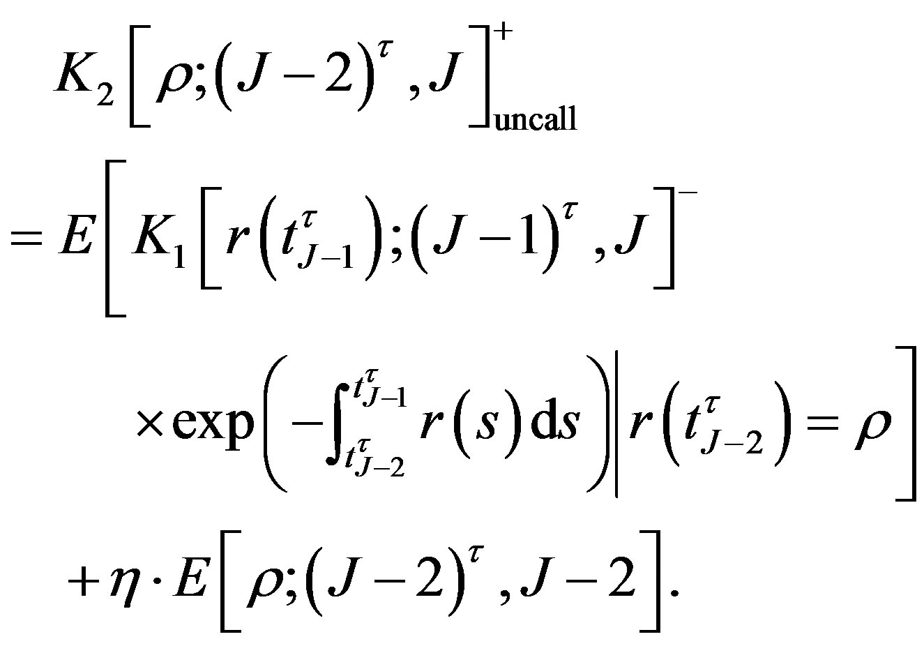 (9)
(9)
Combining the expression (9) we have
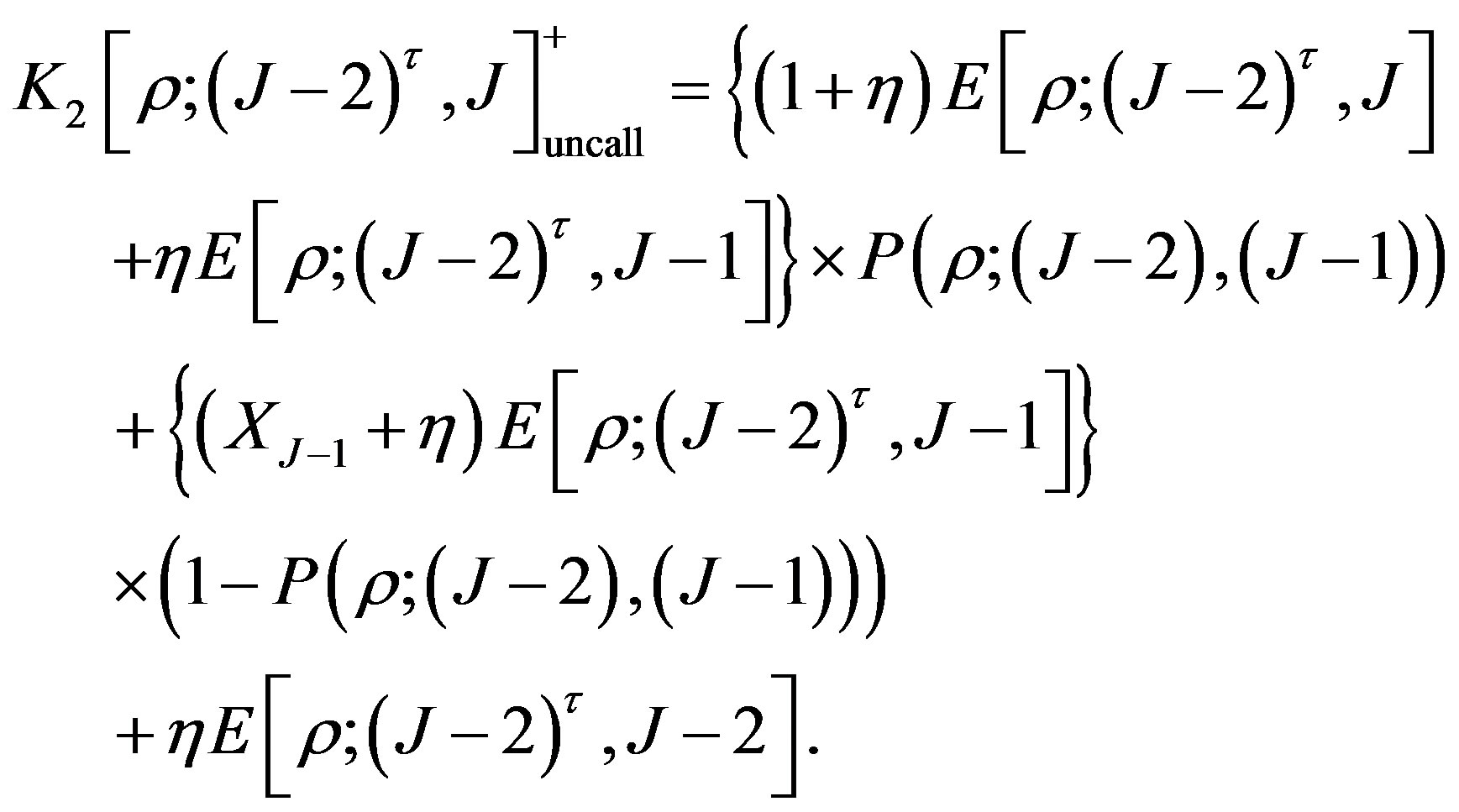 (10)
(10)
On the other hand, if the bond is called, under the given condition: , the value is given by
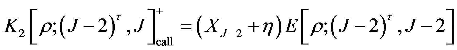 , (11)
Therefore, the bond value at the second notice date  is given by
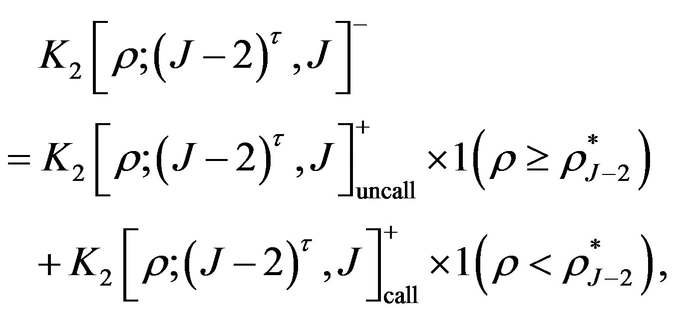 (12)
(12)
where  is the break-even interest rate at the second notice date
 , which can be found as the first breakeven interest rate
 .
.
Continuously, we can obtain the values of callable bond at the jth notice date  as
as
 (13)
(13)
where  is the break-even interest rate at the jth notice date
 .
.
Consequently, we get the price of the callable bond at the present date  with the initial interest rate
  :
:
 (14)
(14)
Now, by applying the simulation technique to the interest rate  and using the Monte Carlo method to approximate the corresponding integrals
  and the corresponding probabilities
 , we can obtain a numerical approximation of the price
  .
.
4. Numerical Experiments
In this section, we do numerical experiments via our methods to price a callable bond issued by the Swiss Confederation with an annual coupon of 4.25%. Here  is December 23, 1991, and
  is December 31, 2012. The protection period is 10 years until year 2002. The notice period is two months. And the call prices are
  ,
,  ,
,  ,
,  ,
,  and
and , respectively.
From [3], the model parameters for the CIR model are ,
,  ,
, . The initial interest rate
 , and the price of straight bond is 0.8114. The break-even interest rates are
 ,
,  ,
,  ,
,  ,
,  and
and , which are given in [3]. Although the break-even interest rates can be obtained via our methods by Equation (6), the results are lack of precision. Therefore we use the results from [3] directly and these break-even interest rates are computed by Equation (7).
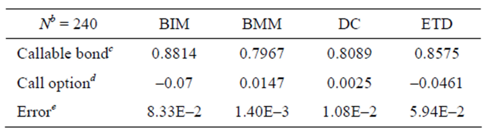
Table 1. Numerical results for four methodsa.
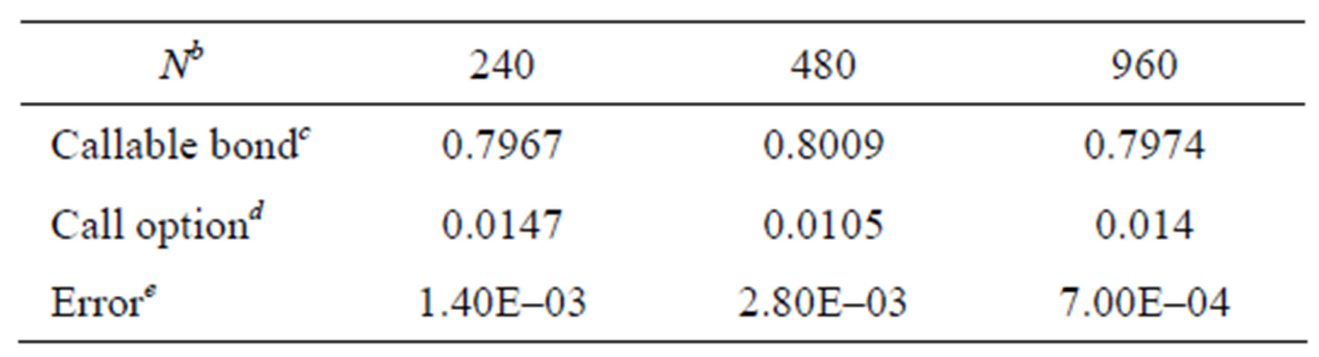
Table 2. Numerical results for different Ns via BMM methoda.
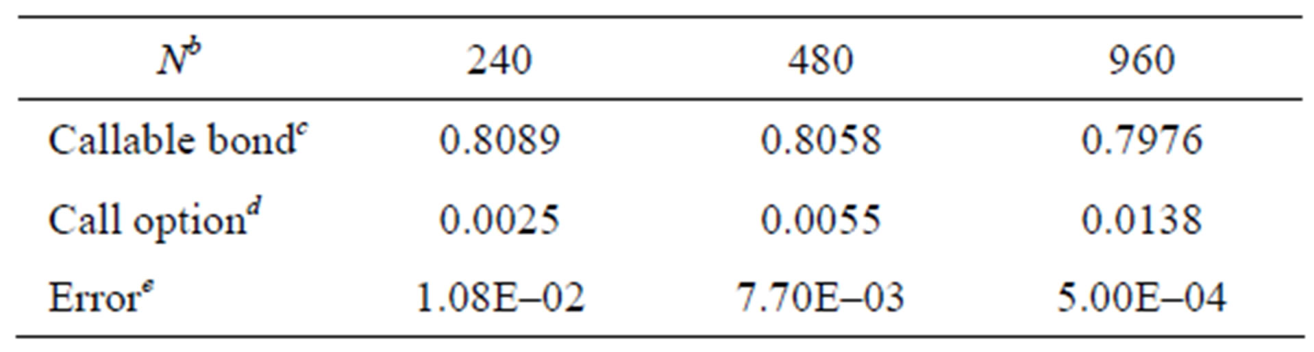
Table 3. Numerical results for different Ns via DC methoda.
aAll prices of callable bond are computed by the average over 50,000 simulating paths.
bN is the number of time-discretized points in the simulation of interest rate.
cAll figures for the callable bond are rounded to four significant digits from the 15-digit results.
dAll prices of the embedded call option all per face value.
eError is the absolute difference between callable bond price and 0.7981, which is given in [3].
Tables 1-3 give the price of this callable bond via different simulation methods. All results in the numerical experiments show that BMM and DC schemes are more efficient than others. And the Monte Carlo method works very well for pricing callable bonds.
5. Acknowledgements
The authors thank the Research Committee of University of Macau for supporting their work (MYRG136(Y1-L2)- FST11-DD, SRF023/09-10S/11T/SYC/FBA).
REFERENCES
- Z. L. Zheng and C. F. Kang, “Pricing and Hedging of Chinese Interest Rate Derivatives,” Peking University Press, Beijing, 2006.
- H.-J. Buttler, “Evaluation of Callable Bonds: Finite Difference Methods, Stability and Accuracy,” The Economic Journal, vol. 105, no. 429, 1995, pp. 374-384. doi:10.2307/2235497
- H.-J. Buttler and J. Waldvogel, “Pricing Callable Bonds by Means of Green’s Function,” Mathematical Finance, vol. 6, no. 1, 1996, pp. 53-88.
- Y. D’Halluin, P. A. Forsyth, K. R. Vetzal and G. Labahn, “A Numerical PDE Approach for Pricing Callable Bonds,” Applied Mathematical Finance, vol. 8, no. 1, 2001, pp. 49-77. doi:10.1080/13504860110046885
- J. Farto and C. V’azquez, “Numerical Techniques for Pricing Callable Bonds with Notice,” Applied Mathematics and Computation, vol. 161, no. 3, 2005, pp. 989- 1013. doi:10.1016/j.amc.2003.12.079
- H. Ben-Ameur, M. Breton, L. Karoui and P. L’Ecuyer, “A Dynamic Programming Approach for Pricing Options Embedded in Bonds,” Journal of Economic Dynamics and Control, vol. 31, no. 7, 2007, pp. 2212-2233. doi:10.1016/j.jedc.2006.06.007
- G. N. Milstein, E. Platen and H. Schurz, “Balanced Implicit Methods for Stiff Stochastic Systems,” SIAM Journal on Numerical Analysis, vol. 35, no. 3, 1998, pp. 1010-1019. doi:10.1137/S0036142994273525
- C. Kahl and H. Schurz, “Balanced Milstein Methods for Ordinary SDEs,” Monte Carlo Methods and Applications, vol. 12, no. 2, 2006, pp. 143-170. doi:10.1515/156939606777488842
- P. Glasserman, “Monte Carlo Methods in Financial Engineering,” 2nd edition, Springer, New York, 2004.
- D. Ding and C. I. Chao, “An Efficient Numerical Scheme for Simulation of Mean-Reverting Square-Root Diffusions,” Journal of Numerical Mathematics and Stochastics, vol. 1, no. 1, 2009, pp. 45-55.
- O. Vasicek, “An Equilibrium Characteriaztion of the Term Structure,” Journal of Financial Economices, vol. 5, no. 2, 1977, pp. 177-188. doi:10.1016/0304-405X(77)90016-2
- J. C. Cox, J. E. Ingersoll and S. A. Ross, “A Theory of the Term-Structure of Interest Rates,” Econometrica, vol. 53, no. 2, 1985, pp. 385-408. doi:10.2307/1911242
NOTES
*Corresponding author.