International Journal of Geosciences
Vol.5 No.6(2014), Article ID:46224,23 pages DOI:10.4236/ijg.2014.56058
Large-Scale Structure Formation via Quantum Fluctuations and Gravitational Instability*
Fernando Porcelli, Giancarlo Scibona
Department for Innovation in Biological, Agro-Food and Forest Systems (DIBAF), University of Tuscia, Viterbo, Italy
Email: porcelli@unitus.it
Copyright © 2014 by authors and Scientific Research Publishing Inc.
This work is licensed under the Creative Commons Attribution International License (CC BY).
http://creativecommons.org/licenses/by/4.0/


Received 27 March 2014; revised 22 April 2014; accepted 12 May 2014
ABSTRACT
This is a review of the status of the universe as described by the standard cosmological model combined with the inflationary paradigm. Their key features and predictions, consistent with the WMAP (Wilkinson Microwave Anisotropies Probe) and Planck Probe 2013 results, provide a significant mechanism to generate the primordial gravitational waves and the density perturbations which grow over time, and later become the large-scale structure of the universe—from the quantum fluctuations in the early era to the structure observed 13.7 billion later, our epoch. In the single field slow-roll paradigm, the primordial quantum fluctuations in the inflaton field itself translate into the curvature and density perturbations which grow over time via gravitational instability. High density regions continuously attract more matter from the surrounding space, the high density regions become more and more dense in time while depleting the low density regions. At late times the highest density regions peaks collapse into the large structure of the universe, whose gravitational instability effects are observed in the clustering features of galaxies in the sky. Thus, the origin of all structure in the universe probably comes from an early era where the universe was filled with a scalar field and nothing else.
Keywords:Large-Scale Structure, Cosmic Inflation, CMB, Non-Gaussianity

1. Introduction
In the past, at the onset of its history, the early universe was hot and dense, a plasma of nuclei, electrons and photons whose mean free path for Thomson scattering was very short. In this universe there is no classical space-time, there is the impassable curvature and density singularity which emerges in the general relativity when the scale factor a approaches zero. A crucial point the zero, a point of infinite density, where what become before the big bang is yet unknown.
At the Planck time, ~10−44 s after the big bang, there are two unique parameters: Planck’s mass and length
 ,
, .
.
At these scales, where the Planck density is  the continuum tears and the space-time itself ends, all known physics comes to halt, physical observables associated with both matter and geometry diverge and quantum gravity becomes necessary. At such very high density its effects become dominant, and then the predictions of the general relativity, based on the space-time as a smooth continuum, are inapplicable in a regime where space and time may be discrete, and quantum effects dominate.
As the universe expanded and cooled down at the recombination era temperature of ~3000˚K, the primordial plasma coalesced into atoms, the photons begin their travel through the universe for 13.7 billion years and their wavelength stretched at the scales of the observable universe. Today, the radiation is observed as cosmic microwave background (CMB), and its measurement, together with the distribution of galaxies, distances to type Ia supernova explosions and others, have revealed that the universe, whose spatial curvature is found to be negligible, is filled with photon, baryons (4%), dark matter (23%) and dark energy (73%).
In our universe, the large-scale structure formation via gravitational instability demands the preexistence of small fluctuations on large physical scales, as galaxies scales ~1 Mpc ~ 1024 cm, which left the Hubble horizon in the radiation and matter dominated eras. However, since at these scales there are no causal mechanisms to generate fluctuations, the generation of primordial small perturbations, at scales smaller than the horizon, and their Gaussianity or non-Gaussianity, are crucial questions for the large classes of cosmological models.
At the present, the six parameters Lambda Cold Dark Matter (ΛCDM) model—the simplest of the Standard Cosmological Models [1] -[6] —is the main stone, but the small fluctuations have to be put in by hand, whereas in the inflationary scenario [7] -[31] there are primordial energy density perturbations correlated to the quantum fluctuations of the inflaton field  which, once the universe became matter dominated (z ~ 3200), were amplified by gravity and grew into the large structures of our universe [29] .
The existence of these primeval inhomogeneities has been confirmed by the Cosmic Background Explorer (COBE) discovery of the cosmic microwave background (CMB) temperature anisotropies which trace back to the inflation lasting different time intervals in different regions of the universe. Inflation then provides a mechanism to generate, not only the density perturbations which later grow into the large-scale structures, but also gravitational waves.
Today, the inflationary potential had become an indispensable building block of the Standard cosmological theory and can be also considered as part of an extension of the Standard Model (SM) of particle physics that is supposed to describe the fundamental interactions at the level of field theory. If the combination these models will survive the current and future cosmological observations, is likely to be the one chosen by Nature. Thus, the origin of all structure in the universe probably comes from an early era where the universe was filled with a homogeneous scalar field  -the inflaton field—and nothing else.
In this early era, the potential  dominated the energy density of the universe decreasing slowly with time as the field
  rolled slowly down its potential slope. The inflaton field perturbation has practically zero mass and negligible interaction. The Fourier components
  of the primordial density perturbation are uncorrelated and have random phases, and the primeval perturbation is Gaussian. The spectrum of the spatial curvature,
  defined as the expectation value of
  at the epoch of horizon exit, defines all of its stochastic properties. The shape of the spectrum is defined by the spectral index
  given as [23]
 . (1.1)
In some models of inflation,  is almost constant on cosmological scales, and the curvature and the gravitational spectra, whose features provide the possibility to be observed, are defined as
 . (1.2)
In the slow-roll inflation the spectrum  is slowly varying, corresponding to a spectral index
  The primordial spectrum
  is also slowly varying and the gravitational wave amplitude is predicted to be GaussianIn this review we try to explain how the primeval inhomogeneity have been generated in the initial moments of the early universe, where a heuristic quantum field—the inflaton—was the source of negative pressure and accelerated expansion. In this short inflation stage
  tiny quantum fluctuations in the inflaton field translated in the density perturbations which, as seeds, grew into of the large-scale structure observed today. In other terms, the quantum fluctuations of the inflaton field were excited during inflation and stretched to cosmological scales. At the same time-since the inflaton fluctuations coupled to the metric perturbations via Einstein’s equations
  -ripples on the metric were also excited and stretched to cosmological scales. Thus, in the cosmic inflation, since perturbations in the inflaton field
  imply perturbations of the energy-momentum tensor,
  and the perturbations of this tensor imply perturbations in the metric
 , both inflaton field and metric perturbations, tightly coupled to each other, lead to the formation of the large-scale structure.
This review, in which many technical details have been suppressed or simplified, is organized as follows: in Section 2, we revise the key features of the standard cosmological model, the ekpyrotic/cyclic models, the slow-roll inflation model with simple polynomial potentials, the loop quantum cosmology (LQC), which deeply modifies the Einstein equations, replaces the singularity with a quantum bounce and extends the inflationary scenario all the way to the Planck regime. In Section 3, we show how the primordial quantum fluctuations and density perturbations grow via gravitational instability to become the large-scale structure of the universe. In Section 4, we relate the key features and predictions of the large classes of models to the current observations—the WMAP and Planck datasets. In Section 5, we reassume the status of large-scale formation via primordial quantum fluctuations and gravitational instability, revise some of the unsolved fundamental questions, as the origin of the inflaton field, and finally conclude that today, the deepest mysteries of our universe is yet the puzzle of whence it came.
2. Cosmological Models
2.1. A Partial List of Available Models
In the development of the inflationary scenario, there are many interesting models: the axion in inflationary cosmology [32] , the hybrid inflation [33] , the eternal self-reprodution chaotic inflationary universe [34] , the inflationary multiverse [29] [35] , the chaotic inflation in supergravity [36] [37] , the string and brane inflation [38] - [41] and others. But, the key features of these heuristic models are still under debate.
The alternatives to the inflationary scenario: pre-big bang [42] [43] , textures and cosmic structures [44] , string gas scenario [45] -[47] , bounce in quantum cosmology [48] , let unsolved one, or more, problems of the standard cosmological model. The same ekpyrotic/cyclic scenario [49] -[51] , introduced as a radical alternative to the standard inflationary cosmology, has its own problems and is yet under debate.
Anyway, the inflationary paradigm is not the only to provide a mechanism for the generation of cosmological perturbations. Other mechanisms have been proposed: the warm scenario [52] [53] , where dissipative effects provide the radiation production occurring in the inflationary expansion stage, the curvaton mechanism [54] -[56] to generate an initially adiabatic perturbation deep in the radiation era, the D-cceleration [57] , an unconventional mechanism for slow roll inflation, the Ghost inflation [58] , where the ghost condensate is a physical field with physical fluctuations, the ekpyrotic/cyclic scenario [49] -[51] , where the field  runs back and forth the interbrane potential
  from some positive value to-∞ and back and the big bang singularity disappears in the endless sequence of epochs, and others.
In the same inflationary scenario there are more than hundred inflation models, where many models provide a mechanism to generate Gaussian and non-Gaussian fingerprints in the early universe whose nature is analyzed in [5] [7] [59] . If the primordial fluctuations are Gaussian-distributed, they are characterized by their power spectrum or, equivalently, by their two-point correlation function. The non-Gaussianity (NG) of the primeval fluctuations is captured by the 3-point correlation function, or its Fourier counterpart, the bispectrum. Different NG configurations (Equilateral, Local, Folded, Orthogonal) are linked to different mechanisms for the generation of non-Gaussian perturbations at different scales.
Here, we just mention few models with detectable amplitude of non-Gaussianity.
Equilateral NG: the single field inflation with a non-canonical kinetic term [60] [61] , the k-inflation [60] [62] , the Dirac-Born-Infeld inflation (DBI) [63] [64] , the general higher-derivative interactions of the inflaton field as ghost inflation [58] .
[There are two types of DBI inflation models. In the UV model the inflaton slides down the potential from the UV side of the warped space to the IR end. This results in a power law inflation when the scale of the potential is high enough. In the IR model, the inflaton is originally trapped in the IR region through some sort of phase transition and then rolls out from the IR to UV side. The resulting inflation is exponential and the potential scale is flexible.]
Folded or flattened NG: the single field with non Bunch-Davies vacuum (NBD) [60] [65] , effective field theories models [66] . Orthogonal NG: Non-Gaussianity in single field inflation [67] ; Local NG: multi-field inflation [68] .
The comparison between the current and future cosmological observation and the predictions and key parameters of these large classes models will decide their fate. Today, the Wilkinson Microwave Anisotropies Probe (WMAP) [69] -[71] and Planck 2013 [72] -[74] datasets have already ruled out some models and strongly constrained others.
2.2. The Standard Cosmological Models
The six parameters ΛCDM model describes successfully many features of the evolution of the universe—the Hubble expansion, the existence of a CMB with a blackbody spectrum, the primordial D, 3He and 7Li abundance, the sum of the masses of the three families of neutrinos, the dark energy equation of state parameter, the number of effective relativistic species, the big bang nucleosynthesis. But, the small fluctuations—which left the Hubble horizon in the radiation and matter dominated eras—have to be put in by hand. Moreover, the model requires that the energy density of the universe has to be tuned near the critical density with an accuracy of 10−55, and postulates the homogeneity and isotropy of the early universe, which must extend to scale beyond the causal horizon at the Planck time.
The standard model then, requires unnatural initial conditions at the big bang, is limited to those epochs where the universe is cool enough to be described by physical processes well established and let unsolved several fundamental problems: the homogeneity, isotropy and flatness of the universe, the origin of irregularities leading to the formation of galaxies and galaxy structures, the primordial monopole gravitino and initial singularity, the about 60 order of magnitude between the Planck’s length (10−33 cm) and mass (10−5 g), and the actual size (1028 cm) and mass (1055 g) of the universe, the vacuum energy problem, which trace back to the idea that the constant scalar field  appearing in unified theories of elementary particles could play the role of a vacuum state with energy density
  in cosmology.
2.3. The Ekpyrotic-Cyclic Universe Scenario
In the ekpyrotic/cyclic scenario [49] -[51] , there are no initial conditions, a bouncing universe replaces inflation, the singularity disappears in the endless sequence of epochs and non-Gaussianities of the local type are produced. In [49] [50] , the scalar field  runs back and forth the interbrane potential
  from some positive value to-∞ and back. In each cycle there is a sequence of kinetic energy, radiation matter and dark energy dominated phases of evolution that agree with the standard big bang cosmology, but the models are not free of conjectures and the key features of the brane world physics are still an open question.
At the present, the cyclic universe [49] [50] faces the question of the metastability of the Higgs vacuum, suggested by the recent measurement at the LHC. (The discovery of a Higgs-like particle with mass 125 - 126 Gev, combined with measurements of the top quark mass, implies that the electroweak Higgs vacuum may be metastable and only maintained by an energy barrier of height h (1010-12 Gev)4 that is well below the Planck density [75] ). The Higgs metastability makes problematic for the big bang to end one cycle, bounce, and begins the next. However, on using an appropriate Weyl-invariant version of the standard model coupled to gravity to track the Higgs evolution in a regularly bouncing cosmology, has been found that exists a band of solutions which solve the problem. The Higgs field escapes from the metastable phase during each big crunch, pass through the bang into an expanding phase, and returns to the metastable vacuum, cycle after cycle. Further, due to the effect of the Higgs, the infinitely cycling universe is geodesically complete, in contrast to inflation where a metastable Higgs makes inflation more improbable [75] .
2.4. Inflationary Scenario
The old [10] and new inflation [13] -[16] have introduced a significant innovation in the Standard Cosmological theory, but in their frameworks there are postulates which are somewhat artificial. The universe, assumed as relatively homogeneous and large enough to survive until the start of the inflation, was in a state of thermal equilibrium from the very beginning; the inflation was an intermediate stage of its evolution. The introduction of the chaotic inflation [17] [18] , which describe the evolution of an universe filled with a chaotically distributed scalar field  resolved all problems of the old and new inflation. In this model, inflation begins in absence of thermal equilibrium and may occur, not only in the models with simple polynomial potentials as but also in any model where the potential has a sufficiently flat region, which allows the existence of the slow-roll regime. In the simplest model of the chaotic inflation with potential
  the value of the scalar field
  determines the existence of different regimes [17] [18] [31] . At energy density of the field
  there is no classical space-time, and then an universe which emerges from the singularity, or from nothing, has to be in a state with Planck density
  which can be described as a classical domain.
In this classical space-time domain, the initial sum of the kinetic energy, gradient energy, and potential energy densities cannot be greater than the Planck density
 , (2.1)
and the expected typical initial conditions are [31]
 (2.2)
(2.2)
In this context, the onset of inflation occurs at the natural condition  and its continuation requires
  within the Planck time.
In the inflation stage, the scalar field  runs its potential from
  to its minimum value. At high potential energy density, the quantum fluctuations of the scalar field
  are large and may lead to an eternal process of self-reproduction of the inflationary universe. At lower values of
  the inflaton field
  slowly rolls down its potential and its fluctuations are small. Finally, near the minimum of
  the field
  rapidly oscillates, loses its energy creating pairs of elementary particles, and the universe becomes hot.
2.5. Cosmic Inflation
In the cosmic inflation with potential , the universe evolution and the inflaton dynamics—in the Friedmann-Lemaitre-Robertson-Walker (FLRW) metric—are governed by the Einstein-Friedmann equations [28]
 (2.3)
(2.3)
 (2.4)
(2.4)
 , (2.5)
where  for an open, flat or closed universe respectively, and the term
  acts as a friction term which slows down the motion of the field
  In an universe governed by these equations, an inflation stage requires a negative pressure, that is
  (Equation (1.4)) as in the de Sitter stage.
For a homogeneous universe  the above simplifies as
 , (2.6)
where 

Therefore, for initially large values, the Hubble parameter was also large—which implies that the friction term  was very large—and the field was moving very slow. At the onset of inflation, the energy density of the scalar field remained almost constant and the expansion of the universe was very fast. Soon after the onset of this regime the conditions

 were satisfied, and then the universe was governed by a simplified system of equations
 . (2.7)
In this inflationary regime, if the field  changes slowly, the size of the universe grew exponentially,
  ,
,  and inflation ended when
 . Solution of these equations states that after a long period of inflation the universe initially filled with the field
  grows exponentially as
  [28] .
In this inflationary paradigm a sufficient slow-roll period is achieved only if the scalar field  is in a region where the potential is sufficiently flat. The flatness condition on the potential is conveniently parametrized in terms of two slow-roll parameters built from the derivatives
 of the potential V with respect to
 . (2.8)
Therefore, to achieve a successful period of inflation these slow-roll parameters must be much smaller than one,  The parameter
  can be also written as
  thus it quantifies the rate of the Hubble parameter H during inflation.
In summary, in the simplest inflation with potential , the realistic value of the mass m is about
  (in Planck units), the total duration of inflation is ~10−30 seconds after the Planck time, and in this very short period the total amount of inflation achieved from the onset of inflation at
  is of the order
 . Inflation ends when the scalar field begins to oscillate near the minimum of
  loses its energy by creating pairs of elementary particles which interact between them and come to a state of thermal equilibrium— the matter creation and reheating stages. From this time on, the universe can be described by the standard cosmological model. An universe whose is many order of magnitude greater than the part of the universe which is today seen,
  cm [31] .
The inflationary paradigm solves many problems of the Standard cosmological models and predicts the existence of inflationary perturbations which serve as seeds which grow into a large scale structure. Therefore, since the detailed features of these perturbations have been observed in the CMB, the predictions of the inflationary scenario appear in agreement with observations However, despite its successes, the inflationary paradigm is conceptually incomplete in several respects. The initial conditions are postulated [76] , the Trans-Planckian issues are ignored [77] , the inflationary space-time is past incomplete, and then inherit the big bang singularity [78] , even though the inflaton violates the standard energy conditions of the singularity theorems [79] .
2.6. Loop Quantum Cosmology
In loop quantum cosmology (LQC) framework [80] -[90] , based on the key features of loop quantum gravity (LQG) [91] -[98] and its underlying Riemannian quantum geometry, space-time and perturbations are quantum, the quantum fields corresponding to the perturbations propagate on a quantum space and the non-perturbative quantum corrections dominate the evolution in the Planck regime, replace the big bang singularity with a quantum bounce and disappear in the low energy regime insuring agreement with the classical general relativity. Thus, the LQC quantum corrections solve the singularity and the ultraviolet-infrared tension: the short distance limitations of classical general.
The LQC novel results are encoded in the modified Einstein-Friedmann equation [87] [100]
 (2.9)
(2.9)
where  and
and  are respectively the Hubble rate and the maximum energy density. This equation for
 , that is away from the Planck regime, reduces to the classical Friedmann equation
 , (2.10)
where for matter density positive,  cannot vanishes, so that every solution represents a contracting, or an expanding universe, whereas in LQC, where the modifications in the Planck regime are drastic,
  vanishes at the quantum bounce
 , to its past the solution represents a contracting universe with
  and to its future, an expanding universe with
 .
.
In LQC, the bounce is an effect of the quantized geometry. The quantum effects act as an effective quantum repulsion, allow the universe to bounce back from a collapse, and then resolve the singularity without fine tuning initial conditions.
From the modified Friedmann equation, and the standard conservation law, it follows that also the deceleration equation is modified to
 . (2.11)
This result implies that, since  can be positive, inflaction (in presence of an appropriate scalar field) is generic in LQC and does not require unlikely initial conditions.
Moreover, the LQC pre-inflationary dynamics of natural conditions at the bounce [101] -[104] , allows to include quantum gravity regime in the standard inflationary scenario, to extend the evolution all the way from deep Planck regime, to ignore the back reaction also in the pre-inflationary epoch, to solve the trans-Planckian problem and to account for the inhomogeneities seen in the CMB, which are the origin of the large scale structure. In the LQC application, for the LFWR space-time with quadratic potential  [100] [104] , the LQC predictions in the low energy regime agree with those of the standard inflationary paradigm: both are compatible with the power spectrum and the spectral index reported in the seven years WMAP data.
Thus, in the low energy regime, LQC and standard inflationary paradigm predictions, compared with the cosmological observation, have the same fate. But, their predictions for the state at the onset of inflation are different: in the standard inflation scenario the onset state is the Bunch-Davies vacuum, while in the LQC pre-inflationary dynamics is the non-Bunch-Davies vacuum [104] .
LQC. Perturbations dynamics on quantum geometry In loop quantum cosmology, the phase space of gauge invariant perturbations is spanned by 3 canonically conjugate pairs representing: one the Mukhanov-Sasaki  and two the tensor modes
 ,
, . In co-moving momentum space they are represented by
 . (2.12)
Therefore, on using the Mukhanov-Sasaki variables  and the two tensor modes denoted by
 , the quantum fields
  and
and  propagate on quantum FLRW geometries which are all regular, free of singularity. A key difference with respect to the standard inflation where the fields propagate on a classical Friedmann solution
 ,
, . Thus, by construction, the framework encompasses the Planck regime and resolves the transPlanckian problem. The evolution equation for tensor modes is given by [104]
 (2.13)
where  is the momentum conjugate to
 ,
,  ,
,  are c-numbers derived from the 4th order adiabatic regularization that depends only on
  and
and 
 are respectively the dressed scale factor and conformal time.
Inflation and slow roll inflation in LQC In LQC [99] [100] , where quantum geometry effects modify the Einstein equations, the Hamiltonian constraint (Equation (2.9)) must be satisfied at any instant of time and the equations of motions given in terms of the variables ,
,  provide the evolution
 (2.14)
 (2.15)
At scales far away from the Planck scale, the quantum effects vanish, the Hamiltonian constraint reduces to the classical Friedmann equation
 , (2.16)
and the slow-roll parameters are given by two distinct sets of parameters
 . (2.17)
In the context of inflationary models, the WMAP7 data [70] —parameterized assuming that the onset of inflation is in the BD vacuum—are tailored to the co-moving mode (or wave number)  given by
 (2.18)
where  is the today scalar factor and
  the mode that has just reentered the Hubble radius today. Within each inflationary model the WMAP data (amplitude of the scalar power spectrum, spectral index) constrains the initials values of field describing the homogeneous isotropic background at time
  at which the co-moving mode
  exits the Hubble radius during the slow-roll stage and the LQC modifications to general relativity are highly suppressed.
At this time  the amplitude
  of the scalar power spectrum
  the spectral index
  the Hubble parameter H and radius
  are
are
 (2.19)
Further, considering the model with quadratic potential,  the equation of motion of the scalar field (Equation (2.13)) simplifies to
 . (2.20)s
For this potential,  the value of the slow-roll parameter at the time
  is given by
 , and at the inflaton
 , its time derivative, the mass m, and the slow-roll parameter
  have the following values [100]
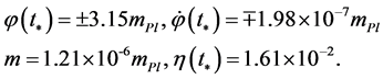 (2.21)
This data leads to the slow-roll inflation with ~50 - 60 e-folding starting at .
.
In LQC pre-inflationary dynamics [104] , at the bounce time  the value of the background inflaton
  is constrained in the interval
  and a solution to the dynamical equations which enters the slow-roll compatible with the seven years WMAP data [70] in its evolution, is obtained for each
  value. The numerical solutions show that for
 , none of the modes that are in the observational range will encounter a significant curvature during their pre-inflationary evolution, and then there are no significant excitations over the BD vacuum at the onset of inflation. On the other hand, if
 , the quantum state at the onset of the slow-roll inflation would carry excitations over the BD vacuum (non-Bunch-Davies vacuum) in modes that are observable in the CMB, where the k0 mode in the range
  that were in the non-BD vacuum leaved their fingerprints—the bispectrum NG flattened configuration.
The LQC scalar power-spectrum  is related to the standard inflationary power-spectrum
  with
with  as the state at onset of inflation
 , (2.22)
where the Bogoliubov coefficients  and
and  are functions only of
  and
and  represents the number density of the BD excitations with momentum
  per unit co-moving volume contained in the state
 . For modes with lower k values, the LQC power-spectrum has a highly oscillatory behavior and differs from the standard power spectrum
  while for reference mode used in the WMAP data
 , the LQC and the standard inflationary predictions are almost the same.
In the standard slow-roll inflation scenario, a significant result is the relation between the tensor-to-scalar ratio  and the tensor spectral index
 . In LQC, the ratio
  does not depend on the pre-inflationary dynamics, and then
  while the tensor spectral index
  is modified in the Planck regime. In [104] , numerical simulations have shown that the imprint left by the pre-inflationary dynamics is potentially observable: a deviation from the standard inflation prediction at low k values.
In summary, LQC and inflationary paradigm predictions are the same in the low energy regime, but drastically differ at Planck scales. Therefore, only the comparison of their key features with the cosmological observations can distinguish between the two, i.e., the excitation over the Bunch-Davies state, non-Gaussianities of the halo bias and the  type distortions in CMB.
3. Quantum Fluctuations and Density Perturbations
3.1. Inflation and Cosmological Perturbations
In the inflationary scenario the universe is described by the FLRW solution to Einstein’s equations with a scalar field as matter source, together with small inhomogeneities that are approximated by a first order perturbation. Fourier modes of quantum fields with co-moving wave number  in the range
  are supposed to be initially in the Bunch-Davies vacuum and its quantum fluctuation, soon after any mode exits the Hubble radius, are assumed to behave as a classical perturbation which evolve according to linearized Einstein’ equations. The existence of inflationary perturbation implies that there must be tiny inhomogeneities at the surface of last scattering, and that they serve as seeds which grow into a large scale structure.
In the simplest inflationary model [31] [41] , the average amplitude of the fluctuations (of all wavelengths) of the field  generated by the inflation during a typical time interval
  is given by [41]
 . (3.1)
The amplitude of these fluctuations,  since the Hubble parameter
  changes very slow in the inflationary stage, remains almost unchanged for a very long time. Therefore, since the wavelength
  of fluctuations
  depends exponentially on the inflation time,
  the spectrum of inhomogeneities
  is almost independent of
  on a logarithmic scale
  and then is a flat spectrum [41] —HarrisonZeldovich spectrum.
In general, since the field fluctuations  lead to a local time delay,
  of the end of inflation,
  a local delay of expansion leads to a density increase in a region of the space,
  , while the density decreases in the regions where the expansion lasts more time. The field fluctuations
  then, lead to density perturbations that via gravitational instability become later large-scale structures. The amplitude of these perturbations is defined as [5] [12] [41]
 . (3.2)
A definition whose derivation is oversimplified since in the inflation stage H and  should be calculated at different time for perturbations with different momentum k. But, in the simplest inflation model with potential
 , where the field
  changes very slowly during inflation, the quantity
  remains almost constant over exponentially large range of wavelengths, and then the spectrum of density perturbations is flat and its amplitude is given by [41]
 . (3.3)
In the simplest inflation model, the perturbations on scale of horizon were produced at  [28] . Hence, using COBE normalization
  the value of m is
 , in Planck units. An exact value of m depends on
 , which in its turn depends slightly on the thermal history of the universe. In short, in the single field slow-roll paradigm, the quantum fluctuations in the inflaton field itself translate, via the Einstein’s equation, into the curvature and density perturbations which grow over time via gravitational instability.
3.2. Quantum Fluctuations and Density Perturbations
In the cosmic inflation, large scale inhomogeneities are related to the restructuring of the vacuum state due to the exponential expansion of the universe. Inflation converts short-wavelength quantum fluctuation  of the scalar field
  into long-wavelength fluctuations, and when the wavelength
  (k momentum) of a fluctuation
  exceeds the horizon
  size, its amplitude is “frozen in” and its nonzero value
  at the horizon crossing is fixed by the damping due to the friction term
  (Equation (2.6)). The amplitude of the fluctuation on super-horizon scales remains unchanged for a very long time, whereas its wavelength keeps growing exponentially [3] . The appearance of such frozen fluctuations is equivalent to the appearance of a classical field
  that does not vanish after having averaged over some macroscopic interval of time. Finally, when the wavelength of these fluctuations reenters the horizon, at some radiation or matter dominated epoch, the curvature (gravitational potential) perturbations, R, of the space-time give rise to matter (and temperature) perturbations
  via the Poisson equation.
The curvature perturbations are a combination of gravitational potential  and energy density perturbations
  [59]
[59]
 (3.4)
(3.4)
where, using the perturbed Einstein equation
 , (3.5)
the first order (linear)  and the second order (non-linear)
  contribution to the gravitational potential are given by
 . (3.6)
Adiabatic perturbations produce a net perturbation in the total energy density and, through the Einstein equations, in the intrinsic spatial curvature. However, as noted in [59] , energy density and curvature perturbations are not gauge-invariant, hence a gauge-invariant variable,  , can be used to define such perturbations. For purely adiabatic perturbations the curvature perturbation is conserved on large scales, and then
  is appropriate to characterize the amplitude of adiabatic perturbations. At second order the curvature perturbation
  on large scales evolves due to non-adiabatic pressure perturbations.
The uniform energy density curvature perturbation  is related to the comoving curvature perturbation
  by
by
 , (3.7)
and then on large scales .
.
In the single-field  slow-roll models of inflation, where the intrinsic entropy perturbation of the inflaton field is negligible on large scales, the power-spectrum of the curvature perturbation on large scales is given by [59]
 (3.8)
(3.8)
where the asterisk stands for the epoch in which a perturbation mode  leaves the Hubble horizon
  during inflation and the spectral-index of the curvature perturbation to lowest order in the slow-roll parameters,
  ,
,  , is
, is
 . (3.9)
The power spectrum of gravity-wave mode  is given by
 , (3.10)
where  is the tensor spectral-index. Therefore, since the fractional change of the power-spectra with scale is much smaller than unity, the power-spectra can be considered as constant on scales relevant for the CMB anisotropy and the tensor—to-scalar amplitude ratio can be defined as
 . (3.11)
For  or
or , given in [105] , the upper bound on the energy scale of inflation is given by [59]
 (3.12)
In summary, in the single field slow-roll scenario, the density perturbations due to the quantum fluctuations in the inflaton field itself translate, via the Einstein’s equations, into the curvature and density perturbations which grow over time via gravitational instability. High density regions continuously attract more matter from the surrounding space, the high density regions become more and more dense in time while depleting the low density regions. At late times the highest density regions peaks collapse into the large structure of the universe, whose gravitational instability effects are observed in the clustering features of galaxies in the sky.
Inflationary dynamics then, explain the formation of all structure in our universe: from primordial quantum fluctuations to large-scale structure. In this context, since large classes of models indicate the inflationary mechanism as responsible of generation of the curvature fluctuations (Gaussian and adiabatic) on super horizon scales, the power spectrum of the curvature perturbations, its spectral-index,  , and the tensor—to-scalar amplitude ratio, r, allow to compare their predictions and key parameters with the current cosmological observations—the Wilkinson Microwave Anisotropy Probe (WMAP) and Planck datasets.
3.3. Fluctuation Dynamics and Power Spectra
The quantum fluctuations in the inflaton and in the transverse and traceless part of the metric, which are amplified by the exponential expansion, yield the scalar and tensor primordial power spectra. In the simple formalism, given in [106] -[108] and used in [74] , the gauge-invariant variable Q describes the inflaton fluctuation  in the uniform curvature gauge. The evolution of its mode function is governed by the equation
 , (3.13)
where  and k is the comoving wave number of the Fourier mode under consideration. The gaugeinvariant field fluctuation is related to the co-moving curvature perturbation
 , which at large scales is related to the uniform energy density curvature perturbation ζ:
 .
.
In a like approach, the gravitational waves are described by two polarization states  of the transverse traceless part of the metric fluctuations amplified by the exponential expansion. The evolution equation for their mode function is given by
 . (3.14)
The above linearized equations, since the primordial perturbations are small, of order 10−5, provide a satisfactory description for the generation and evolution of perturbations in the inflation stage, from the sub-Hubble to super-Hubble evolution.
The power spectra of curvature and tensor perturbations on super-Hubble scales, yielded by the primordial quantum fluctuations in the inflaton and in the transverse traceless part of the metric, are defined as [74]
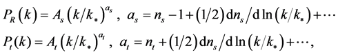 (3.15)
where ,
,  are the scalar and tensor amplitude,
  ,
,  are the scalar and tensor scalar index, the derivatives
 ,
,  are the running of the scalar and tensor spectral index and the asterisk stands for the value of the inflaton field
  at which the mode
  crosses the Hubble radius for the first time.
In the single field slow-roll approximation, the number of e-folds before the end of inflation,  at which the pivot scale
  exits the from the Hubble radius, is
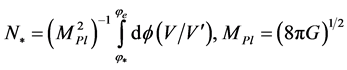 , (3.16)
where prime denotes derivatives with respect to the field , and subscript e denotes the end of inflation. The scalar and tensor amplitude,
  and spectral index,
  , are given by [74]
 (3.17)
where the tensor to scale modes ratio r and the slow-roll parameters,  ,
,  , are
, are
 (3.18)
3.4. Alternative, Equivalent Definitions
In [69] , the quantity  closely related to the amplitude,
  of the primordial curvature perturbations
 , is considered as a powerful and practical tool to test significant features of a large class of models which predict that
  is nearly a power law
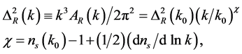 (3.19)
where  gives an approximate contribute of
  (at a given scale per logarithmic interval in k) to the total variance of
 , as
, as , while the spectral index
  and the spectral index
  are used to define the tilt of the spectrum and the running index. For
  and
and  the power-law spectrum is a pure Harrison-Zeldovich “scale invariant spectrum”, while for
  this spectrum is strongly disfavored.
The primordial gravitational waves, predicted by many cosmological models, leaves their signatures imprinted on the CMB temperature anisotropy (the tensor E-mode, B-mode and TE-mode polarization) [69] . The amplitude and power spectrum of these gravitational waves, since gravity is encoded in the metric, are defined as
 (3.20)
where  is the power spectrum of tensor metric perturbations, hk, the amplitude is given as
  and the amplitude, in the form of the tensor
  to scalar
  ratio, r, is defined as [69] [70]
 (3.21)
which is used to calculate the tensor mode contributions to the B-mode, E-mode and TE power spectra. The spectral index  and the ratio r are related to the inflation slow-roll parameters, and then can be used to constraint the inflationary models [23] [69]
 , (3.22)
 (3.23)
where  is the reduced Planck mass, and the derivatives are evaluated at the mean value of the scalar field
  at the time that a given scale leaves the Hubble horizon. The combination of these two equations relates
  and r
and r
 . (3.24)
This equation, since r is correlated to both  and the curvature of the potential allows to distinguish models on the
  plane and justify the use of the sign and magnitude of the potential curvature to classify inflation models [69] .
In the period of cosmic inflation, the generated quantum fluctuations, as explained in (3.2), became the seeds for the cosmic structures observed today. In this contest, inflation models predict that the primordial fluctuations is nearly a Gaussian distribution with random phase. This prediction is based on the assumption that the probability distribution of quantum fluctuations,  of the free scalar field
  in the Bunch-Davies vacuum is a Gaussian distribution, so that also the probability distribution of primordial curvature perturbations, R, generated by the field
  would be a Gaussian distribution. Therefore, deviations from a Gaussian distribution, as nonGaussian correlations in the primordial curvature perturbations, is a significant test of the inflation predictions.
Today, the WMAP and Planck results, and the non-Gaussianity (NG) of the primordial fluctuations, captured by the bispectrum different configurations (local, equilateral, folded, orthogonal), are the most important information used to rule out or constrain the 193 inflation models available [109] [110] .
3.5. The Bispectrum
The primordial curvature perturbation, R, cannot be measured directly, a more observable quantity is the curvature perturbation during the matter era,  written in the local form
 , (3.25)
where  which represents the gravitational potential at linear order, is correlated to the linear part of the curvature perturbation,
 is the “local nonlinear coupling parameter”, and both sides of the equation are evaluated at the same location in space [69] [70] .
The amplitude of non-Gaussian correlations can be evaluated using the angular bispectrum of CMB temperature anisotropy, the harmonic transform of the 3-point correlation function. The observed angular bispectrum is related to the 3-dimensional bispectrum of primordial curvature [73]
 , (3.26)
where the potential  equivalent to the Bardeen’s gauge-invariant gravitational potential is defined in terms of the co-moving curvature perturbation ζ on super-horizon scales by
 . The bispectrum
  measures the correlation among three perturbation mode and, for translational and rotational invariance, it depends only on the magnitude of the three wave-vectors
 , (3.27)
where the “nonlinearity” parameter,  , is a dimensionless parameter which measures the amplitude of NG.
3.6. Non Gaussian Configuration
Different NG configurations are linked to different mechanisms for the generation of non-Gaussian perturbations at different scales, where the primeval inflaton field interactions, encoded in the three wave numbers,  , are captured by signal peaking in triangles of different form: Orthogonal, Local, Equilateral, Folded, [73] .
Orthogonal NG, which generate a signal with a positive peak at the equilateral configuration and a negative peak at the folded configuration [69] .
Local NG , where the signals peaks in squeezed triangles, which occurs, not only when the primordial NG is generated on super-horizon scales, as in the multi-field inflation models [111] -[113] and in a new bouncing cosmology [114] , but also when enhanced NG is generated by the modified non-Bunch-Davies (NBD) vacuum initial state, as in the excited canonical single-field inflation [115] .
Equilateral NG triangular configuration of the three comoving momentum vectors  due to correlation between fluctuation modes of comparable wavelength, which occurs if the three perturbation modes cross the horizon at approximately the same time.
Examples of this class include: single field with non-canonical kinetic term [60] [61] , k-inflation [62] , DiracBorn-Infeld (DBI) inflation [63] [64] , models with higher-derivative interactions of the inflaton field as ghost inflation [58] , effective field theory models [116] .
Folded NG, where the signal peaks in flattened triangles , which occurs when the primordial NG is generated by the initial state, where the inflaton field interactions are stronger at the onset of inflation than at the end, and then there is enhanced NG coming from excited initial state in the early inflation stages.
Examples of this class include: single field models with non-Bunch-Davies (NBD) vacuum [61] [65] , models with general higher-derivative interactions [68] , excited canonical single-field inflation model with modified NBD initial state whose enhanced bispectrum has two leading order shapes [115] : the single-field NBD1 squeezed configuration and the single-field NBD2 flattened configuration which differ from the much flattened non-Bunch-Davies (NBD) bispectrum  [61] . These shapes are typically oscillatory since are regularized by a cutoff scale
  giving the oscillatory period. This cutoff,
  where
where  is the speed of the sound of inflaton fluctuations, is determined by the finite time
  in the past when the NBD component was initially excited.
Anyway, all these bispectrum differ from that for single-field inflation models with a Bunch-Davies vacuum initial state, particularly the NBD1 squeezed shape whose wave number  is of importance for observations [117] .
[The BD vacuum is a state tailored to a few e-folding before the mode  leaves the Hubble horizon; in this state the physical length of the mode
  equals the radius
  of the observable universe at the surface of last scattering].
Thus, the bispectrum defined in Equation (3.27) measures 1) the fundamental self-interactions of the scalar field (or fields) involved in the inflation, as well as 2) their interactions which generate the primordial curvature perturbations, and also 3) the non-Gaussianity—the quantities 

 —which represent the higher order perturbations occurring during or after the inflation. Therefore, it brings insights into the physics behind inflation, as the pre-inflationary dynamics of the loop quantum cosmology [104] .
4. Cosmological Models and Current Observations
4.1. The WMAP and Planck Probes Observations
Today, the Wilkinson microwave anisotropies probe (WMAP) data [69] -[71] , the Planck measurements of the cosmic microwave background (CMB) [72] -[74] , and their search of non-Gaussianity in the distribution of dark matter and galaxies in the late universe allow to compare the key parameters and predictions of many cosmological models with the observational data.
In the inflationary scenario the CMB, whose amplitude of tensor B-mode polarization is proportional to the energy of inflation and tied to the range of inflaton field, is the unique window between the late-time universe and the early universe at the time of the potential energy domination that drove cosmic inflation. The phenomenology of non-Gaussianity in the distribution of dark matter and galaxies allows to study the dynamics of inflation. It is then clear that a wide range of cosmological data plays an essential role 1) in testing the large classes of model and their predictions and 2) in constraining their key parameters.
4.2. The WMAP Datasets: ΛCDM Model
In the standard cosmological model (ΛCDM), based on a flat expanding universe whose constituents are dominated by cold dark matter (CDM) and a cosmological constant (Λ) at late times, the dynamics is governed by general relativity and the primordial seeds of structure formation are nearly scale-invariant adiabatic Gaussian fluctuations.
The six key parameters of the simplest ΛCDM model have proven to be a satisfactory fit to nine years WMAP data alone, or combined with the latest distance measurements from baryon acoustic oscillation (BAO) in the distribution of galaxies, the Hubble parameter H0 measurements, and the extended CMB data (eCMB) which include the Atacama Cosmology Telescope (ACT) and the South Pole Telescope (SPT) data. Here we report only the nine years WMAP combined (WMAP + eCMB + BAO + H0) data given in ([71] , Table 2).
ΛCDM parameters
The given WMAP results show that the six parameters ΛCDM model describes all the data remarkable well, and there are no evidence for deviations from this model: the geometry of the observable universe is flat and the dark energy is consistent with a cosmological constant. The amplitude of matter fluctuations,  , is consistent with all existing data, including cluster abundance, peculiar velocity, and gravitational lensing. The simplest ΛCDM model then, survived the most stringent nine years WMAP test.
Beyond the ΛCDM parameters, the combined (WMAP + eCMB + BAO + H0) data exclude a scale invariant primordial power spectrum at  significance. In addition to adiabatic fluctuations, where all species fluctuate in phase and then produce curvature fluctuations, isocurvature perturbations producing no net curvature are possible. These entropy, or isocurvature perturbations—occurring when an over-density in one specie compensate the under-density in another—have a measurable effect on the CMB shifting the acoustic peaks in the power spectrum. But, no significant contribution from these perturbations has been detected in the nine year WMAP data, whether or not additional data have been included in the fit.
4.3. The WMAP Datasets: Inflation Models
In the combined (WMAP + eCMB + BAO + H0) data for a power-law spectrum of primordial curvature perturbations
 , (4.1)
With  the power-law spectral index, without B-mode polarization measurements—that is ignoring tensor mode, is
 (4.2)
(4.2)
The tightest constraint on tensor modes r (Equation (4.3)) and on the running scalar index  from the nine year WMAP combined data are [71]
 . (4.3)
Therefore, the current data strongly disfavor a pure Harrison-Zeldovich spectrum, also if tensor modes are included in the model fits.
In the large classes of inflation models, the WMAP data [71] well support the predictions of single-field inflation models for features of primordial curvature: the temperature fluctuations, which linearly trace the primordial curvature perturbations are adiabatic and Gaussian [118] . The limits on primordial gravitational waves are consistent with many inflation models, including the Starobinsky model [8] with spectral index  and tensor to scalar ratio r given by
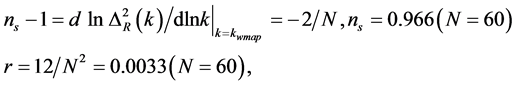 (4.4)
(4.4)
where N is the number of e-folding related to  and r. The non-Gaussian features of primordial fluctuations in inflationary models [29] [30] has not been evidenced. In general, since an analysis of the CMB maps [118] has shown that all the quantities

 does not differ significantly from zero, there is no compelling evidence for deviations from Gaussianity. Hence, inflationary models predicting the existence of no-Gaussianity are strongly disfavored by the WMAP results.
The two dimensional joint marginalized constraints (68%, 95%) on the primordial tilt  allows to constrain and distinguish inflation models on
  plane [70] . In this class of models, as reported in [69] , the single-field inflation models with chaotic potential
  with
with ,
,  have different fate. The model with potential
  is far away from the 95% region for both N = 50 and 60, and then is excluded at more than 99% CL. The inflation model with potential
  lies outside of the 68% region for N = 50, while for N = 60 is at the boundary of this region. Hence the model is under pressure.
In conclusion, the six parameters ΛCDM model and the single-field inflation models for Gaussian features of primordial curvature survived the most stringent WMAP tests.
4.4. The Planck Datasets
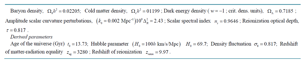
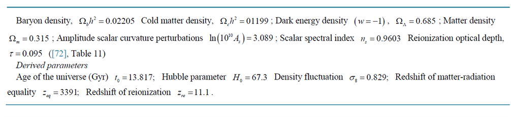
In the Plank 2013 results [72] the most important conclusion is that the Planck temperature power spectrum at high multipoles  agrees with the predictions of the six-parameter ΛCDM model. Here we report only the (Plank + WP 68% limits) data given in ([72] , Table 2, Table 11 for
 ).
).
ΛCDM parameters (Planck)
The Planck data show that the simplest ΛCDM model provides a good match to the Planck power spectrum of the lensing potential,  and to the TE and EE power spectra at high multipoles, but no in the low multipoles range
  This mismatch, and other anomalies at low multipoles, although not of decisive significance for the model, imply that it may be incomplete.
Moreover, in the Planck 2013 data given in ([72] , Table 11) the low value of the nine years WMAP Hubble parameter, H0 = 74 ± 11, with respect the Planck + WP H0 = 65.2 ± 1.8, and a high matter density, Ωm = 0.315 ± 0.016 are in tension. Therefore, as noted in [119] , if the tension between previous measurement of H0 and that recently derived by the Planck team within the assumptions of a six-parameter flat ΛCDM model (including tension with WMAP 9), cannot be resolved by unknown systematics, it will force the rejection of the six-parameter model in favor of a more complex alternative.
However, despite these limits, the six parameters ΛCDM model has proven to be successful in describing a wide range of cosmological data, including the Type Ia supernovae magnitude-distance relation, baryon acoustic oscillation measurements, the large-scale clustering of galaxies and cosmic shear, and its predictions have been confirmed but the nine years WMAP and Planck 2013 results. Hence, the tension between the WMAP and Planck data are not a compelling evidence of its incompleteness. Other observations are needed to decide about its limits.
4.5. The Planck Datasets: Non-Gaussianity
In the Planck results 2013 [73] , dedicated to constraints on primordial non-Gaussianity, the final results

 and
and

 (4.5)
(4.5)
show that there is no evidence for primordial NG in these shapes. Therefore, the models predicting the non Gaussianity of the primeval perturbations via these bispectrum shapes are strongly disfavored or constrained.
Here, we give a partial list of models. 1) For the non Bunch-Davies models with flattened bispectral often in combination with non trivial squeezed limit, which can be generated by strong disturbance away from background slow-roll evolution or additional trans-Planckian physics [61] [65] [115] [120] , there is no convincing evidence for the predicted bispectra and the related non-Gaussianity of the primordial perturbations. The same results hold for the non-Bunch-Davies resonant models.
2) Warm Inflation [52] [53] produce a related shape with a sign change in the squeezed limit. The resulting bispectrum has no evidence for significant correlation with Planck data.
3) In the ekpyrotic/cyclic scenarios [49] -[51] the “ekpyrotic conversion” mechanism has been ruled out and the parameter space of the “kinetic conversion” mechanism significantly limited.
However, as noted in [73] , the results for the non-Bunch-Davies (NBD) models are just preliminary. A systematic search for best-fit Planck NBD models using the parameter freedom available has to be undertaken.
Anyway, a possible explanation for the non-detection of the non-Gaussianity in the NBD models is given in [121] for open inflation. The amplitude of the bispectrum is exponentially suppressed in the sub-curvature region for wavelengths shorter than the today curvature radius, and so the non Bunch-Davies effect of open inflation on the observable bispectrum is exponentially suppressed.
4.6. The Planck Datasets: Cosmic Inflation
In the Planck 2013 results [74] , dedicated to the status of cosmic inflation, the scalar amplitude As and the scalar spectral index ns (adding a tensor component) for the primordial curvature perturbations spectrum (Equation (3.15)) are
 , (4.6)
a  departure from
  The tightest constraint on tensor modes r and on the running scalar index
  are
are
 . (4.7)
Here, we just mention some of the more than hundred inflationary models [110] .
1) In the Planck 2013 results for cosmic inflation [74] , the simplest slow-roll single field  inflation survived an exacting test with the Planck data. The spatial curvature
  at 95% CL and the bispectral non-Gaussianity parameter
  consistent with zero are compatible with the zero spatial curvature and small value of
  as predicted in this simplest slow-roll single field model.
2) The axion monodromy potentials,  and
and  models [109] [122] are the most compatible with the Planck data, while the
  model is decisively ruled out, the large quadratic potential and natural inflation, are somewhat disfavored by the Planck data, when broader entropy generation scenarios are considered.
3) Other models with an exponential potential, a monomial potential with a power larger than two, or hybrid model driven by a quadratic term are disfavored at more than 95% CL. The axion and curvaton scenario in which the isocurvature mode is uncorrelated or fully correlated with the adiabatic mode, are disfavored by Planck data. The IR DBI (Dirac-Born-Infeld) inflation, k-inflation, inflation involving gauge fields and warm inflation have been strongly constrained. In the ekpyrotic/cyclic scenarios the “ekpyrotic conversion” mechanism has been ruled out and the parameter space of the “kinetic conversion” mechanism strongly limited.
In summary, in the simplest versions of the chaotic inflation with  for
for  the predictions of the inflationary models with
  are consistent with the Planck data, the simplest quadratic potential is marginally consistent, whereas the
  model is ruled out. In the chaotic inflation in super-gravity [123] the predictions of the model with potential
 (4.8)
(4.8)
are in agreement with the Planck data. Therefore, as noted in [123] , a slight modification of the simplest chaotic inflation with a quadratic potential leads to a model consistent with the Planck 2013 results.
A Long list of other models compatible with the Planck data is given in [124] where, besides the Bayesian analysis of the inflationary models consistency with the Planck results, is noted that the models consistent with the Planck results cannot be considered as “true” models, they are the simplest and most effective inflationary hypothesis compatible with the Planck 2013 CMB data.
Before to conclude this section, we recall the predictions of the loop quantum cosmology and discuss their consistency with the Planck 2013 data.
In the LQC application, for the simplest slow-roll inflation with potential  [100] [104] , the LQC and the simplest inflation model predictions are the same in the low energy regime, but strongly differ at the Plank scale. In the simplest inflationary paradigm, the state at the onset of inflation state is the Bunch-Davies vacuum. In the LQC pre-inflationary for
  at the bounce the quantum state at the onset of the slowroll inflation is the non-bunch-Davies vacuum [104] .
Therefore, since in the Planck 2013 results on the non-Gaussianity [73] there is no evidence for primordial non-Gaussianity (Equation (4.4)), the LQC pre-inflationary dynamics predictions  are not consistent with the Planck data, but for
  its key features and predictions are compatible with the observations.
Hence, this LQC specific application for the inflation with  is under pressure for its pre-inflationary dynamics predictions, but the novel features of the loop quantum cosmology—space and time discrete at the Planck scale, the modified Einstein equation (Equation (2.9)) which replace the singularity with a quantum bounce, and others—are still significant and innovative.
However, as noted in [73] , the results for the non-Bunch-Davies (NBD) models are just preliminary. A systematic search for best-fit Planck NBD models using the parameter freedom available has to be undertaken.
In conclusion, the Planck 2103 data for non Gaussianity and for inflationary models (Equations (4.6), (7)), including the Bayesian consistency, are not definitive since future observations can change the constraint limits. Therefore, models that are disfavored or severely constrained by the current Planck data can be favored, or more disfavored, by future observation, i.e., in ([73] , p. 10): “The model with a quadratic potential, n = 2 (Linde, 1983), often considered the simplest example for inflation, now lies outside the joint 95% CL for N 60 e-folds”.
5. Cosmological Models: Unsolved Fundamental Questions
5.1. The Status of our Universe
Today, the six-parameters ΛCDM model and the simplest slow-roll single field  inflation, which are the most effective hypothesis compatible with the WMAP and Planck 2013 data, provide a convincing description of the status of our universe and of the large-scale formation via primordial quantum fluctuations and gravitational instability. The ΛCDM model describes successfully many features of the evolution of the universe—the Hubble expansion, the existence of a CMB with a blackbody spectrum, the primordial D, 3He and 7Li abundance, the sum of the masses of the three families of neutrinos, the dark energy equation of state parameter, the number of effective relativistic species, the big bang nucleosynthesis.
In the single field slow-roll paradigm, the density perturbations due to the quantum fluctuations in the inflaton field itself translate, via the Einstein’s equations, into the curvature and density perturbations which grow over time via gravitational instability. High density regions continuously attract more matter from the surrounding space, the high density regions become more and more dense in time while depleting the low density regions. At late times the highest density regions peaks collapse into the large structure of the universe, whose gravitational instability effects are observed in the clustering features of galaxies in the sky. Thus, the origin of all structure in the universe probably comes from an early era where the universe was filled with a heuristic scalar field  generated by the vacuum fluctuations during inflation, and nothing else.
5.2. The Unsolved Questions
The inflationary paradigm has successfully explained the generation of primordial perturbation and of gravitational waves. However, despite its successes, it is conceptually incomplete in several respects. The inflationary space-time is past incomplete, and then inherit the big bang singularity. The initial conditions are specified at the onset of inflation and then evolves the quantum perturbations, but at the onset of inflation the curvature is some 10−11 - 10−12 times the Planck scale. Thus, what really happened at the Planck regime is bypassed. Another question is the quantum to classical transition [125] -[127] . The inflationary physics replaces the quantum state of perturbations with a Gaussian statistical distribution of classical perturbations, but what happens physically is not explained.
Furthermore, the inflationary paradigm, as well as the ΛCDM model and also the loop quantum cosmology, does not tell where the inflaton with mass-energy above 1012 Gev comes on, nor how the potential arise. The hypothesis of its generation from vacuum fluctuation does not explain what physically happens in the early era. A crucial question then the origin of the inflaton, a question closely related to the problem of the origin of our universe, but its solution is beyond the existing theories. In the same Standard Model of particles physics, whose 26 free parameters justifies that is only a low energy effective theory, an approximation, an outstanding question is “why our universe is matter dominated”, “what is its origin?” [128] .
In our days, the available understanding of the physical world is fragmented, leaves unanswered fundamental questions, and then the need of a new synthesis is the great challenge of fundamental physics. It is not then a case, if on the crucial question of the universe origin the relativistic and quantum cosmological theories are still confined in the old paradigms—the eternal, endless sequence of epochs and the quantum creation from nothing. Today, the deepest mysteries of our universe is yet the puzzle of whence it came [129] .
6. Conclusions
In our days, we live in an unusual time, perhaps a golden age of the cosmology. The impressive cosmological observations and measurements have revealed, not only that the observable part of the universe is nearly flat, filled with photon, baryons (4%), dark matter (23%) and dark energy (73%), but also that the expansion of the universe is accelerating: a pair of galaxies separated by a million light years are drifting apart at a velocity of 68 kilometers a second as the universe expands. An universe then, that is expanding more faster than in the past and consists primarily of mysterious exotic substances, defined generically as dark matter and dark energy since their real nature is yet unknown. These observations have deeply changed the key features of the universe and put under pressure many of the more than hundred cosmological models available.
The WMAP and Planck 2013 results have already ruled out many models and significantly constrained others. Their severe screening of large classes of models has ruled out the inflationary  model and others, marginalized the simplest quadratic potential model, disfavored the ekpyrotic/cyclic model, already under strong pressure after the discovery of the universe acceleration and the detection of primordial gravitational waves, and favored both the six-parameters ΛCDM model and the simplest slow-roll single field
  inflation, which have survived their stringent tests.
Thus, in the landscape of more than hundred model, the standard cosmological model combined with the single field  inflationary model is one the most effective hypothesis which provides a convincing description of the status of the observable universe and of the large-scale formation via primordial quantum fluctuations and gravitational instability.
The cosmological observations then, have significantly restricted the number of models compatible with their datasets and, beyond their tests on different classes of models, have deeply affected the development of new cosmological theories. Their main purpose is no more the construction of hypothesis and models to describe and predict large local non-Gaussianity, but the elaboration of new models of inflation capable to fit their predicted data in the  plane provided by the current and future cosmological observations, as WMAP, Planck and others.
In conclusion, the standard cosmological model and the simplest single field  slow-roll inflation well-fit the current WMAP and Planck 2013 datasets. Thus, if this combination will survive future observations, is likely to be the one chosen by Nature: the more than 350 millions cosmic structure, catalogued in the SDSS (Sloan digital sky survey) and others archives, come from an early era where the universe was filled with a scalar inflaton field
  and nothing else. Future observations will decide the fate of this heuristic conclusive hypothesis.
References
- Weinberg, S. (1972) Gravitation and Cosmology. John Wiley & Sons, Hoboken.
- Peebles, P.J.E. (1980) The Large-Scale Structure of the Universe. Princeton University Press, Princeton.
- Peebles, P.J.E. (1993) Principles of Physical Cosmology. Princeton University Press, Princeton.
- Padmanabhan, T. (1993) Structure Formation in the Universe. Cambridge University Press, Cambridge.
- Mukhanov, V. (2005) Physical Foundations of Cosmology. Cambridge University Press, New York.
- Weinberg, S. (2008) Cosmology. Oxford University Press, Oxford.
- Starobinsky, A.A. (1979) Spectrum of Relict Gravitational Radiation and the Early State of the Universe. JETP Letters, 30, 682-685.
- Starobinsky, A.A. (1980) A New Type of Isotropic Cosmological Model without Singularity. Physics Letters B, 91, 99- 102. http://dx.doi.org/10.1016/0370-2693(80)90670-X
- Mukhanov, V. and Chibisov, G. (1981) Quantum Fluctuation and ‘Nonsingular’ Universe. JETP Letters, 33, 532-535.
- Guth, A.H. (1981) Inflationary Universe: A Possible Solution to the Horizon Flatness Problems. Physical Review D, 23, 347-356. http://dx.doi.org/10.1103/PhysRevD.23.347
- Chibisov, G. and Mukhanov, V. (1982) Galaxy Formation and Phonons. Monthly Notices of the Royal Astronomical Society, 200, 535-550.
- Albrecht, A. and Steinhardt, P.J. (1982) Cosmology for Grand Unified Theories with Radiatively Induced Symmetry Breaking. Physical Review Letters, 48, 1220-1223. http://dx.doi.org/10.1103/PhysRevLett.48.1220
- Linde, A.D. (1982) A New Inflationary Universe Scenario: A Possible Solution of the Horizon, Flatness Homogeneity, Isotropy and Primordial Monopole Problems. Physics Letters B, 108, 389-393. ]http://dx.doi.org/10.1016/0370-2693(82)91219-9
- Linde, A.D. (1982) Coleman-Weinberg Theory and the New Inflationary Universe Scenario. Physics Letters B, 114, 431-435. http://dx.doi.org/10.1016/0370-2693(82)90086-7
- Linde, A. (1982) Temperature Dependence of Coupling Constant and the Phase Transition in the Coleman-Weinberg Theory. Physics Letters B, 116, 340-342. http://dx.doi.org/10.1016/0370-2693(82)90294-5
- Linde, A. (1982) Scalar Field Fluctuation in the Expanding Universe and the New Inflationary Universe Scenario. Physics Letters B, 116, 335-339. http://dx.doi.org/10.1016/0370-2693(82)90293-3
- Linde, A.D. (1983) Chaotic Inflation. Physics Letters B, 129, 177-181. http://dx.doi.org/10.1016/0370-2693(83)90837-7
- Linde, A. (1985) Initial Conditions for Inflation. Physics Letters B, 162, 281-286. http://dx.doi.org/10.1016/0370-2693(85)90923-2
- Mukhanov, V. and Chibisov, G. (1985) Gravitational Instability of the Universe Filled with a Scalar Field. JETP Letters, 41, 493-496.
- Goncharov, A.S., Linde, A.D. and Mukhanov, V.F. (1987) The Global Structure of the Inflationary Universe. International Journal of Modern Physics A, 2, 561-591. http://dx.doi.org/10.1142/S0217751X87000211
- Linde, A.D., Linde, D.A. and Mezhlumian, A. (1994) From the Big Bang Theory to the Theory of a Stationary Universe. Physical Review D, 49, 1783-1826. http://dx.doi.org/10.1103/PhysRevD.49.1783
- Liddle, A.R. (1999) An Introduction to Cosmological Inflation. 36 p. arXiv: astro-ph 9901124v1
- Lyth, D.H. and Riotto, A. (1999) Particle Physics Models of Inflation and the Cosmological Density Perturbation. Physics Reports, 314, 1-146. http://dx.doi.org/10.1016/S0370-1573(98)00128-8
- Liddle, A. and Lyth, D. (2000) Cosmological Inflation and Large-Scale Structure. Cambridge University Press, Cambridge.
- Brandenburger, R.H. (2001) A Status Review of Inflationary Cosmology.
- Guth, A.H. (2004) Inflation.
- Mukhanov, V.F. (2004) CMB Quantum Fluctuations and the Predictive Power of Inflation. International Journal of Theoretical Physics, 43, 623.
- Linde, A.D. (1990) Particle Physics and Inflationary Cosmology. Harwood Academic, Chur.
- Acquaviva, V., Bartolo, N., Matarrese, S. and Riotto, A. (2003) Gauge-Invariant Second-Order Perturbations and NonGaussianity from Inflation. Nuclear Physics B, 667, 119-148. http://dx.doi.org/10.1016/S0550-3213(03)00550-9
- Maldacena, J. (2003) Non-Gaussian Features of Primordial Fluctuations in Single Field Inflationary Models. Journal of High Energy Physics, 2003, 013.
- Linde, A.D. (2008) Inflationary Cosmology. Lecture Notes in Physics, 738, 1-54.
- Linde, A.D. (1991) Axions in Inflationary Cosmology. Physics Letters B, 259, 38-47. http://dx.doi.org/10.1016/0370-2693(91)90130-I
- Linde, A.D. (1994) Hybrid Inflation. Physical Review D, 49, 748-754. http://dx.doi.org/10.1103/PhysRevD.49.748
- Linde, A.D. (1986) Eternally Existing Self-Reproducing Chaotic Inflationary Universe. Physics Letters B, 175, 395- 400. http://dx.doi.org/10.1016/0370-2693(86)90611-8
- Linde, A. (2002) Inflation, Quantum Cosmology and the Anthropic Principle.
- Kallosh, R. and Linde, A. (2003) P-Term, D-Term and F-Term Inflation. Journal of Cosmology and Astroparticle Physics, 2003, 008.
- Linde, A. (2013) Chaotic Inflation in Supergravity and Cosmic String Production. Physical Review D, 88, Article ID 123503.
- Kallosh, R. (2008) On Inflation in String Theory. Lecture Notes in Physics, 738, 119-156.
- Dvali, G.R. and Tye, S.H.H. (1999) Brane Inflation. Physics Letters B, 450, 72-82. http://dx.doi.org/10.1016/S0370-2693(99)00132-X
- Quevedo, F. (2002) Lectures on String/Brane Cosmology. Classical and Quantum Gravity, 19, 5721-5779.
- Linde, A. (2006) Inflation and String Cosmology. Progress of Theoretical Physics Supplement, 163, 295-322. http://dx.doi.org/10.1143/PTPS.163.295
- Veneziano, G. (1991) Scale Factor Duality For Classical and Quantum Strings. Physics Letters B, 265, 287-294. http://dx.doi.org/10.1016/0370-2693(91)90055-U
- Gasperini, M. and Veneziano, G. (1993) Pre-Big-Bang in String Cosmology. Astroparticle Physics, 1, 317-339.
- Spergel, D. and Turok, N. (1992) Textures and Cosmic Structure. Scientific American, 266, 52-59. http://dx.doi.org/10.1038/scientificamerican0392-52
- Nayeri, A., Brandenberger, R.H. and Vafa, C. (2006) Producing a Scale-Invariant Spectrum of Perturbations in a Hagedorn Phase of String Cosmology. Physical Review Letters, 97, Article ID: 021302. http://dx.doi.org/10.1103/PhysRevLett.97.021302
- Brandenberger, R.H., Nayeri, A., Patil, S.P. and Vafa, C. (2007) Tensor Modes from a Primordial Hagedorn Phase of String Cosmology. Physical Review Letters, 98, Article ID: 231302. http://dx.doi.org/10.1103/PhysRevLett.98.231302
- Brandenberger, R.H., Nayeri, A., Patil, S.P. and Vafa, C. (2007) String Gas Cosmology and Structure Formation. International Journal of Modern Physics A, 22, 3621-3642.
- Peter, P., Pinho, E.J.C. and Pinto-Neto, N. (2007) Noninflationary Model with Scale Invariant Cosmological Perturbations. Physical Review D, 75, Article ID: 023516. http://dx.doi.org/10.1103/PhysRevD.75.023516
- Khoury, J., Ovrut, B.A., Steinhardt, P.J. and Turok, N. (2001) Ekpyrotic Universe: Colliding Branes and the Origin of the Hot Big Bang. Physical Review D, 64, Article ID: 123522. http://dx.doi.org/10.1103/PhysRevD.64.123522
- Steinhardt, P.J. and Turok, N. (2005) The Cyclic Model Simplified. Talk Given at Dark Matter 2004, Santa Monica, CA: 18-20 February 2004; New Astronomy Reviews, 49, 43-57.
- Buchbinder, E.I., Khoury, J. and Ovrut, B.A. (2008) Non-Gaussianities in New Ekpyrotic Cosmology. Physical Review Letters, 100, Article ID: 171302.
- Berera, A. (1995) Warm Inflation. Physical Review Letters, 75, 3218-3221. http://dx.doi.org/10.1103/PhysRevLett.75.3218
- Berera, A. (1996) Thermal Properties of an Inflationary Universe. Physical Review D, 54, 2519-2534. http://dx.doi.org/10.1103/PhysRevD.54.2519
- Enqvist, K. and Sloth, M.S. (2002) Adiabatic CMB Perturbation in Pre-Big-bang String Cosmology. Nuclear Physics B, 626, 395-409. http://dx.doi.org/10.1016/S0550-3213(02)00043-3
- Lyth, D.H. and Wands, D. (2002) Generating the Curvature Perturbations without an Inflaton. Physics Letters B, 254, 5-14.
- Morroi, T. and Takahashi, T. (2001) Effects of Cosmological Moduli Fields on Cosmic Microwave Background. Physics Letters B, 522, 215-221.
- Maldacena, J.M. (1998) The Large N limit of Superconformal Field Theories and Supergravity. Advances in Theoretical and Mathematical Physics, 2, 231-252.
- Arkani-Hamed, N., Creminelli, P., Mukohyamam, S. and Zaldarriaga, M. (2004) Ghost Inflation. Journal of Cosmology and Astroparticle Physics, 2004. http://dx.doi.org/10.1088/1475-7516/2004/04/001
- Bartolo, N., Komatsu, E., Matarrese, S. and Riotto, A. (2004) Non-Gaussianity from Inflation: Theory and Observations. Physics Reports, 402, 103-266.
- Chen, X., Huang, M., kachru, S. and Shiu, G. (2007) Observational Signature and Non-Gaussianity of General Single Field. Journal of Cosmology and Astroparticle Physics, 2007. http://dx.doi.org/10.1088/1475-7516/2007/01/002
- Chen, X., Easther, R. and Lim, E.A. (2007) Large Non-Gaussianity in Single Field Inflation. Journal of Cosmology and Astroparticle Physics, 2007. http://dx.doi.org/10.1088/1475-7516/2007/06/023
- Armendáriz-Picón, C., Damour, T. and Mukhanov, V. (1999) K-Inflation. Physics Letters B, 458, 209-218. http://dx.doi.org/10.1016/S0370-2693(99)00603-6
- Silverstein, E. and Tong, D. (2004) Scalar Speed Limits and Cosmology: Acceleration from D-Cceleration. Physical Review D, 70, Article ID: 103505. http://dx.doi.org/10.1103/PhysRevD.70.103505
- Alishahiha, M., Silverstein, E. and Tong, D. (2004) DBI in the Sky: Non-Gaussianity from Inflation with a Speed Limit. Physical Review D, 70, Article ID: 123505. http://dx.doi.org/10.1103/PhysRevD.70.123505
- Holman, R. and Tolley, A.J. (2008) Enhanced Non-Gaussianity from Excited Initial States. Journal of Cosmology and Astroparticle Physics, 2008. http://dx.doi.org/10.1088/1475-7516/2008/05/001
- Chen, X., Easther, R. and Lim, E.A. (2008) Generation and Characterization of Large NG in Single Field Inflation. Journal of Cosmology and Astroparticle Physic, 2008. http://dx.doi.org/10.1088/1475-7516/2008/04/010
- Bartolo, N., Matarrese, S. and Riotto, A. (2010) Non-Gaussianity and the Cosmic Microwave Background Anisotropies. Advance in Astronomy, 2010, Article ID: 157079.
- Vernizzi, F. and Wands, D. (2006) Non-Gaussianity in Two Field Inflation. Journal of Cosmology and Astroparticle Physics, 2006. http://dx.doi.org/10.1088/1475-7516/2006/05/019
- Komatsu, E., et al. (2009) Five-Year Wilkinson Microwave Anisotropy Probe (WMAP) Observations: Cosmological Interpretation. The Astrophysical Journal Supplement Series, 180, 330-376. http://dx.doi.org/10.1088/0067-0049/180/2/330
- Komatsu, E., et al. (2011) Seven-Year Wilkinson Microwave Anisotropy Probe (WMAP) Observations: Cosmological Interpretation. The Astrophysical Journal Supplement Series, 192, Article ID: 18. http://dx.doi.org/10.1088/0067-0049/192/2/18
- Hinshaw, G., Larson, D., Komatsu, E., et al. (2011) Nine-Year Wilkinson Microwave Anisotropy Probe (WMAP) Observations: Cosmological Parameter Results. The Astrophysical Journal Supplement Series, 208, Article ID: 19.
- Planck Collaboration: Ade, P.A.R., Aghanim, N., Armitage-Caplan, C., et al. (2013) Planck 2013 Results. XVI. Cosmological Parameters.
- Planck Collaboration: Ade, P.A.R., N. Aghanim, C., Armitage-Caplan, et al. (2013) Planck 2013 Results. XXIV. Constraints on Primordial Non-Gaussianity. Submitted to Astronomy & Astrophysics.
- Planck Collaboration: Ade, P.A.R., N. Aghanim, C., Armitage-Caplan, et al. (2013) Planck 2013 Results. XXII, Constraints on Inflation. Submitted to Astronomy & Astrophysics.
- Bars, I., Steinhardt, P.J. and Turok, N. (2013) Cyclic Cosmology and the Metastability of the Higgs.
- Brandenberger, R.H. (2011) Introduction to Early Universe Cosmology.
- Brandenberger, R.H. and Martin, J. (2012) Trans-Planckian Issues for Inflationary Cosmology.
- Borde, A., Guth, A. and Vilenkin, A. (2003) Inflationary Space-Time Are Not Past Complete. Physical Review Letters, 90, Article ID: 151301. http://dx.doi.org/10.1103/PhysRevLett.90.151301
- Hawking, S.W. and Ellis, G.F.R. (1973) The Large Scale Structure of Space-Time. Cambridge University Press, Cambridge. http://dx.doi.org/10.1017/CBO9780511524646
- Bojowald, M. (2001) Loop Quantum Cosmology IV: Discrete Time Evolution. Classical and Quantum Gravity, 18, 1071-1088. http://dx.doi.org/10.1088/0264-9381/18/6/308
- Bojowald, M. (2001) Absence of a Singularity in Loop Quantum Cosmology. Physical Review Letters, 86, 5227-5230. http://dx.doi.org/10.1103/PhysRevLett.86.5227
- Bojowald, M. (2001) Dynamical Initial Conditions in Quantum Cosmology. Physical Review Letters, 87, Article ID: 121301. http://dx.doi.org/10.1103/PhysRevLett.87.121301
- Bojowald, M. (2002) Inflation from Quantum Geometry. Physical Review Letters, 89, Article ID: 261301. http://dx.doi.org/10.1103/PhysRevLett.89.261301
- Bojowald, M. (2002) Quantization Ambiguities in Isotropic Quantum Geometry. Classical and Quantum Gravity, 19, 5113-5130. http://dx.doi.org/10.1088/0264-9381/19/20/306
- Bojowald, M. (2003) Homogeneous Loop Quantum Cosmology. Classical and Quantum Gravity, 20, 2595-2615. http://dx.doi.org/10.1088/0264-9381/20/13/310
- Ashtekar, A., Bojowald, M. and Lewandowski, J. (2003) Mathematical Structure of Loop Quantum Cosmology. Advances in Theoretical and Mathematical Physics, 7, 233-268.
- Ashtekar, A. and Singh, P. (2011) Loop Quantum Cosmology: A Status Report. Classical and Quantum Gravity, 28, Article ID: 213001.
- Agullo, I. (2013) Loop Quantum Cosmology.
- Ashtekar, A., Pawlowski, T., Singh, P. and Vandersloot, K. (2007) Loop Quantum Cosmology of k = 1 FRW Models. Physical Review D, 75, Article ID: 024035.
- Ashtekar, A. and Wilson-Ewing, E. (2009) Loop Quantum Cosmology of Bianchi Type II Model. Physical Review D, 80, Article ID: 123532. http://dx.doi.org/10.1103/PhysRevD.80.123532
- Sen, A. (1982) Gravity as Spin System. Physical Review B, 119, 89-91. http://dx.doi.org/10.1016/0370-2693(82)90250-7
- Barbero, F. (1995) Real Ashtekar Variables for Lorentzian Signature Space-Time. Physical Review D, 51, 5507-5510. http://dx.doi.org/10.1103/PhysRevD.51.5507
- Rovelli, C. (1997) Loop Quantum Gravity. Living Reviews in Relativity, 1, 1-74.
- Rovelli, C. (2010) A New Look at Loop Quantum Gravity. Classical and Quantum Gravity, 28, Article ID: 114005. http://dx.doi.org/10.1088/0264-9381/28/11/114005
- Rovelli, C. (2011) Loop Quantum Gravity: The First 25 Years. Classical and Quantum Gravity, 28, Article ID: 153002.
- Ashtekar, A. (1986) New Variables for Classical and Quantum Gravity. Physical Review Letters, 57, 2244-2247. http://dx.doi.org/10.1103/PhysRevLett.57.2244
- Ashtekar, A. (1987) New Hamiltonian Formulation of General Relativity. Physical Review D, 36, 1587-1603. http://dx.doi.org/10.1103/PhysRevD.36.1587
- Ashtekar, A., Kaminski, W. and Lewandowski, J. (2009) Quantum Field Theory on a Cosmological, Quantum SpaceTime. Physical Review D, 79, Article ID: 064030. http://dx.doi.org/10.1103/PhysRevD.79.064030
- Ashtekar, A. and Sloan, D. (2010) Loop Quantum Cosmology and Slow Roll Inflation. Physical Review B, 694, 108- 112.
- Ashtekar, A. and Sloan, D. (2011) Probability of Inflation in Loop Quantum Cosmology. General Relativity and Gravitation, 43, 3619-3656. http://dx.doi.org/10.1007/s10714-011-1246-y
- Agullo, I., Ashtekar, A. and Nelson, W. (2012) A Quantum Gravity Extension of the Inflationary Scenario. Physical Review Letters, 109, Article ID: 251301.
- Agullo, I., Ashtekar, A. and Nelson, W. (2013) Extension of the Quantum Theory of Cosmological Perturbations to the Planck Era. Physical Review D, 87, Article ID: 043507. http://dx.doi.org/10.1103/PhysRevD.87.043507
- Ashtekar, A. (2013) Loop Quantum Gravity and the Planck Regime of Cosmology. 23 p. (Plenary talk at the Conference: Relativity and Gravitation: 100 Years after Einstein in Prague). arXiv:1303.4989
- Agullo, I., Ashtekar, A. and Nelson, W. (2013) The Pre-Inflationary Dynamics of Loop Quantum Cosmology: Confronting Quantum Gravity with Observations. Classical and Quantum Gravity, 30, Article ID: 085014.
- Peiris, H.V., et al. (2003) First-Year Wilkinson Microwave Anisotropy Probe (WMAP) Observations: Implications for Inflation. The Astrophysical Journal Supplement Series, 148, 213. http://dx.doi.org/10.1086/377228
- Mukhanov, V. (1988) Quantum Theory of Gauge Invariant Cosmological Perturbations. Soviet Physics, JETP, 67, 1297-1302.
- Mukhanov, V., Feldman, H. and Brandenberger, R. (1992) Theory of Cosmological Perturbations. Physics Report, 215, 203-233. http://dx.doi.org/10.1016/0370-1573(92)90044-Z
- Sasaki, M. (1986) Large Scale Quantum Fluctuations in the Inflationary Universe. Progress of Theoretical Physics, 76, 1036-1046. http://dx.doi.org/10.1143/PTP.76.1036
- McAllister, L., Silverstein, E. and Westphal, A. (2010) Gravity Waves and Linear Inflation from Axion Monodromy. Physical Review D, 82, Article ID: 046003. http://dx.doi.org/10.1103/PhysRevD.82.046003
- Martin, J., Ringeval, C. and Vennin, V. (2013) Encyclopaedia Inflationaris. 368 p. arXiv:1303.3787
- Lyth, D.H., Ungarelli, C. and Wands, D. (2003) Primordial Density Perturbation in the Curvaton Scenario. Physical Review D, 67, Article ID: 023503. http://dx.doi.org/10.1103/PhysRevD.67.023503
- Bartolo, N., Matarrese, S. and Riotto, A. (2004) Non-Gaussianity in the Curvaton Scenario. Physical Review D, 69, Article ID: 043503. http://dx.doi.org/10.1103/PhysRevD.69.043503
- Zaldarriaga, M. (2004) Non-Gaussianities in Models with a Varying Inflaton Decay Rate. Physical Review D, 69, Article ID: 043508. http://dx.doi.org/10.1103/PhysRevD.69.043508
- Creminelli, P. and Senatore, L. (2007) A Smooth Bouncing Cosmology with Scale Invariant Spectrum. Journal of Cosmology and Astroparticle Physics, 2007. http://dx.doi.org/10.1088/1475-7516/2007/11/010
- Agullo, I. and Parker, L. (2011) Non-Gaussianity and the Stimulated Creation of Quanta in the Inflationary Universe. Physical Review D, 83, Article ID: 063526. http://dx.doi.org/10.1103/PhysRevD.83.063526
- Cheung, C., Fizpatrick, A.L., Kaplan, J., Senatore, L. and Creminelli, P. (2008) The Effective Field Theory of Inflation. Journal of High Energy Physics, 2008. http://dx.doi.org/10.1088/1126-6708/2008/03/014
- Agullo, I. and Shandera, S. (2012) Large Non-Gaussian Halo Bias from Single Field Inflation. Journal of Cosmology and Astroparticle Physics, 2012. http://dx.doi.org/10.1088/1475-7516/2012/09/007
- Bennett, C., Larson, D., et al. (2013) Nine-Year Wilkinson Microwave Anisotropy Probe (WMAP) Observations: Final Maps and Results. The Astrophysical Journal Supplement Series, 208, 20.
- Treu, T., Marshall, P.J., et al. (2013) Dark Energy with Gravitational Lens Time Delays. 9 p. arXiv:1306.1272v1
- Meerburg, P.D., van der Schaar, J.P. and Corasanti, P.R. (2009) Signatures of Initial State Modification on Bispectrum Statics. Journal of Cosmology and Astroparticle Physics, 5. http://dx.doi.org/10.1088/1475-7516/2009/05/018
- Sugimura, K. and Komatsu, E. (2013) Bispectrum from Open Inflation. Journal of Cosmology and Astroparticle Physics, 11. http://dx.doi.org/10.1088/1475-7516/2013/11/065
- Silverstein, E. and Westphal, A. (2008) Monodromy in the CMB: Gravity Waves and String Inflation. Physical Review D, 78, Article ID: 106003. http://dx.doi.org/10.1103/PhysRevD.78.106003
- Linde, A. (2014) Inflationary Cosmology after Planck 2013. 84 p. (Based on Lectures at the Les Houches School “Post-Planck Cosmology”, 2013). arXiv:1402.0526v2
- Martin, J., Ringeval, C. and Vennin, V. (2013) The Best Inflationary Models after Plank. 63 p. arXiv:1312.3529
- Kiefer, C., Polarski, D. and Starobinsky, A.A. (1998) Quantum to Classical Transition for Fluctuations in the Early Universe. International Journal of Modern Physics D, 7, 455-462. http://dx.doi.org/10.1142/S0218271898000292
- Kiefer, C. and Polarski, D. (2009) Why Do Cosmological Perturbations Look Classical to Us? Advanced Science Letters, 2, 164-173. http://dx.doi.org/10.1166/asl.2009.1023
- Sudarsky, D. (2011) Shortcomings in the Understanding of Why Cosmological Perturbations Look Classical. International Journal of Modern Physics D, 20, 509-552. http://dx.doi.org/10.1142/S0218271811018937
- Sliwa, K. (2013) Atlas Overview and Main Results. CERN Document Server: ATL-PHYS-PROC-2013-130. arXiv:1305.4551v1
- Penrose, R. (2011) Cycle of Time. Vintage Books, London.
NOTES

*Quntum Fluctuations and Gravitational Instability.