Advances in Remote Sensing
Vol. 2 No. 2 (2013) , Article ID: 32870 , 9 pages DOI:10.4236/ars.2013.22013
Simulations of Seasonal and Latitudinal Variations in Leaf Inclination Angle Distribution: Implications for Remote Sensing
University of Maryland Baltimore County, Joint Center for Environmental Technology, NASA Goddard Space Flight Center, Greenbelt, USA
Email: karl.f.huemmrich@nasa.gov
Copyright © 2013 Karl F. Huemmrich. This is an open access article distributed under the Creative Commons Attribution License, which permits unrestricted use, distribution, and reproduction in any medium, provided the original work is properly cited.
Received February 28, 2013; revised March 30, 2013; accepted April 6, 2013
Keywords: Leaf Angles; NDVI; fAPAR; Canopy Reflectance Models; Canopy Structure
ABSTRACT
The leaf inclination angle distribution (LAD) is an important characteristic of vegetation canopy structure affecting light interception within the canopy. However, LADs are difficult and time consuming to measure. To examine possible global patterns of LAD and their implications in remote sensing, a model was developed to predict leaf angles within canopies. Canopies were simulated using the SAIL radiative transfer model combined with a simple photosynthesis model. This model calculated leaf inclination angles for horizontal layers of leaves within the canopy by choosing the leaf inclination angle that maximized production over a day in each layer. LADs were calculated for five latitude bands for spring and summer solar declinations. Three distinct LAD types emerged: tropical, boreal, and an intermediate temperate distribution. In tropical LAD, the upper layers have a leaf angle around 35˚ with the lower layers having horizontal inclination angles. While the boreal LAD has vertical leaf inclination angles throughout the canopy. The latitude bands where each LAD type occurred changed with the seasons. The different LADs affected the fraction of absorbed photosynthetically active radiation (fAPAR) and Normalized Difference Vegetation Index (NDVI) with similar relationships between fAPAR and leaf area index (LAI), but different relationships between NDVI and LAI for the different LAD types. These differences resulted in significantly different relationships between NDVI and fAPAR for each LAD type. Since leaf inclination angles affect light interception, variations in LAD also affect the estimation of leaf area based on transmittance of light or lidar returns.
1. Introduction
Vegetation canopies are complex collections of leaves, branches, fruits, and flowers. One of the main purposes of the canopy is to absorb solar radiation to power photosynthesis. The arrangement and quantity of the leaves influence how well light penetrates the canopy, affecting the distribution of light to the leaves. Important canopy characteristics that determine the interception of radiation include:
a) leaf area indexb) vertical distribution of the foliagec) the leaf inclination angle distributiond) leaf optical propertiese) the distribution of the leaves in the canopy, i.e. the clumpiness, and f) leaf azimuth angle distribution [1].
In the organization of the canopy, plants balance light interception against other factors, such as water usage and temperature control [2,3]. The same canopy characteristics determining light interception also affect the spectral reflectance of the canopy providing a link between canopy architecture and remote sensing (e.g. [4, 5]).
Leaf orientation with respect to the position of the sun is a key factor in determining the amount of light intercepted by a leaf, and also affects the fraction of incident sunlight that penetrates the canopy to lower layers of leaves [6,7]. The orientation of a leaf is described by its azimuth and inclination angles. The direction from north that the leaf points in is the azimuth angle, and the leaf inclination angle is a measure of the droop of the leaf from horizontal. Often leaf inclination distributions within a canopy are described by mathematical functions, such as spherical, erectophile, or extremophile [8,9].
Leaf azimuth and inclination angle distribution may vary between plant species, growth stage or even time of day [8,10-14]. Some plants show heliotropic leaf movements, with the leaves tracking the sun throughout the day. A diaheliotropic leaf, one that keeps its surface perpendicular to the direction of the sun, can intercept over 50% more solar radiation than a horizontal leaf over a day. Conversely, a paraheliotropic leaf, one that keeps the leaf surface parallel to the sun, minimizes light interception [15,16]. Leaf angles that reduce light interception can reduce midday heat loads on the leaf and increase water use efficiency [2,3]. Further, since the photosynthetic light response of leaves saturates at moderate light levels [17], leaves that tend to be vertical may maintain high photosynthetic levels during periods of high solar elevations although intercepting less light than horizontal leaves [18]. While at low solar elevations the vertical leaves may have an advantage over horizontal leaves by intercepting more light when the incident light is not saturating [19].
Leaf inclination angles also vary with position in the canopy. Duncan’s [20] modeling study showed that having erect leaves at the canopy top and horizontal leaves in the lower levels of the canopy maximized mid-summer mid-latitude plant photosynthesis. Horn’s [18] model also predicts that leaves at the top of the canopy will tend to be erect, while leaves low in the canopy will tend toward horizontal to maximize photosynthesis. The general results of these modeling studies are supported by observations of forest canopies. Measurements of summertime leaf inclination angles in several mid-latitude temperate forests show the upper canopy mean leaf inclination angles between 35˚ and 55˚ and understory leaf inclination angles around 15˚ [21-24].
When viewed from a point on the Earth, the path the sun takes through the sky over a day depends on the time of the year and latitude of the observer. If canopy leaf inclination angle distributions (LAD) are affected by solar illumination, then the distribution of inclination angles may be related to latitude. Herbert [25] showed that mean leaf inclination angles of the arctic rose (Dryas octopetala L.) increased with decreasing latitude over a wide range of northern latitudes. He also found leaf inclination angles for subtropical species followed the same relationship with latitude as the arctic rose. Bartlett et al. [26] studied salt marsh cord grass (Spartina alterniflora L.) over its range in eastern North America from Nova Scotia at 46˚N south to Florida at 29˚N. They examined relationships between Spectral Vegetation Indices (SVI), such as the Normalized Difference Vegetation Index (NDVI), and biomass and found an abrupt discontinuity in the relationships for cord grass that occurred at approximately 37˚30'N. They attribute the change to differences in leaf angles; northern canopies leaves were more horizontal than the leaves in the southern canopies.
The work of Bartlett et al. [26] points out the importance of considering variations in leaf inclination angles in the interpretation of remotely sensed data. Modeling studies have shown the relationship between NDVI and the daily fraction of absorbed photosynthetically active radiation (fAPAR) to be linear [27] or smooth curves [4, 5,28]. Studies looking at the effect of different LADs found only small variations the NDVI-fAPAR relationship [4,5]. However, these studies used theoretical distribution functions, assumed the leaf angle distribution to be the same throughout the canopy, and did not examine differences in illumination patterns for varying latitudes for different LADs.
LAD is an important structural feature of plant canopies, and one of the more adaptable characteristics, yet little is known if identifiable LAD patterns occur in nature, and, if they do, what their spatial and temporal variability are. For a given location and time, are there optimal LADs? If so, what does the light penetration pattern look like in these LADs? Finally, what effect might varying LAD patterns have on the remote sensing of biophysical variables? This paper tries to make a first attempt to address these questions through a simple “thought experiment” by joining a canopy radiative transfer model with a simple leaf photosynthesis model to predict leaf angle distributions that optimize photosynthesis within canopy layers for a variety of locations and times. The model also allows an examination of the effect of the resulting LADs on the remote sensing of the canopy.
2. Model Description
The SAIL (Scattering from Arbitrarily Inclined Leaves) canopy model is used to simulate the reflectance and absorption of radiation by a vegetation canopy [29,30]. The SAIL model calculates energy fluxes at any depth in the canopy, and can determine a directional reflectance for any combination of sun and view angles. The model assumes a canopy made up of uniform horizontal layers of infinite extent. The characteristics of each layer are determined by the amount, orientation, and optical properties of the materials occurring in that layer. In the model the distribution of the material within each layer is assumed to be random. Leaf azimuth angles are also assumed to be random. In this study the leaf optical properties (i.e. leaf spectral reflectance and transmittance) are held constant throughout the canopy using baseline values from Goward and Huemmrich [5].
For each layer the absorbed photosynthetically active radiation (APAR) is calculated from the energy fluxes above and below that layer. APAR for a given layer is found using the relation:
 (1)
(1)
where PARo is the incoming radiation at the top of the layer, PARr is the radiation reflected upward from the top of the layer, PARi is the radiation transmitted downward through the layer and PARsr is the radiation reflected upward into the layer from lower layers and soil [31]. In the lowest layer of the canopy the term in parenthesis is the radiation absorbed by the soil. The amount of instantaneous APAR is determined from the SAIL model and is a function of how LAD and leaf area index (LAI) for each layer interact with the sun angle. To determine the daily fAPAR APAR values are summed throughout the daylight period and divided by the total incoming PAR for the day [5].
APAR must be determined for each leaf as an input into the photosynthesis model. This is calculated by dividing the total APAR for a layer by the leaf area of that layer. Since this produces an average illumination over the layer, it is important to have low leaf areas within the layer to minimize the effect of shadowing. This study uses layers with a LAI of 0.5. This constraint has no effect on the physical thickness of the layer since the SAIL model has no explicit measurement of depth in it.
A simple relationship between photosynthesis rate and light intensity for a constant carbon dioxide concentration is:
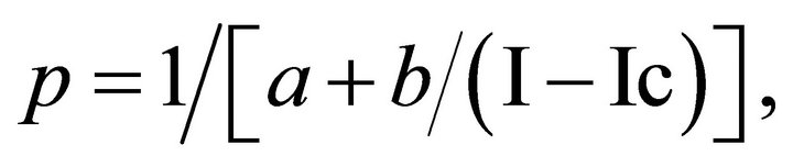 (2)
(2)
where p is the rate of dry matter production in g∙m−2∙hr−1, I is the intensity of solar radiation in W∙m−2, and Ic is the light compensation point [17]. The parameters a and b describe the controlling factors affecting photosynthesis. Under intense light, photosynthesis reaches a maximum value of 1/a. Therefore, a is proportional to the sum of the resistances to carbon dioxide diffusion from the air to the chloroplasts. The term b/I may be regarded as the photochemical resistance, so that b is inversely proportional to the quantum efficiency in low light levels. In this simulation exercise the value of a is taken as 1 m2∙hr∙g−1, b as 34.9 W∙hr∙g−1, and Ic, is 1 W∙m−2. These values remain constant for all layers; that is, there are no sun or shade leaves in the model. Incident solar radiation is assumed to contain 45% of energy in the photosynthetically active region of 0.4 to 0.7 micrometers [32]. The direct beam radiation reaching the surface of the earth is taken to be 1047 W∙m−2. Incident PAR at the canopy top is the product of the total direct beam PAR and the cosine of the solar zenith angle for the given location and time of day. The fraction of diffuse incoming PAR, if any, is also added to the incident PAR.
The photosynthesis model uses the APAR per leaf area determined from the SAIL model as an input to calculate gross production. The instantaneous photosynthesis values are integrated to get daily production. Respiration is not included in the calculations. The model begins with a single layer with an LAI of 0.5 for a given location and day of year (see Figure 1). Leaf inclination angles are varied between 5˚ and 85˚ in 10˚ increments and the daily productivities are compared. The inclination angle with the highest production is saved. The next iteration consists of two layers, where the top layer has a fixed leaf inclination angle of the maximum producer in the previous step. The inclination angles of the lower layer are varied to find the maximum daily production as before. This process is repeated for several layers, stopping if the APAR for the leaves in a layer becomes less than the light compensation point. There is no attempt in the model to maximize total canopy production, but only to maximize the daily production of each layer. This assumption is true if the canopy consists of different plants occupying different canopy layers or if there is little or no transport of photosynthetic production between

Step 1 Step 2 Step 3
Figure 1. A schematic diagram showing the approach used for modeling vertical patterns of leaf inclination angle distribution in vegetation canopies. In Step 1, the modeling begins with a single layer in the SAIL model with an LAI of 0.5 over the soil background. Leaf inclination angles are varied between 5˚ and 85˚ under the range of solar zenith angles that describe the daily path of the sun for a given place and date. Daily productivities for each leaf inclination angle are compared and the inclination angle with the highest production is saved. In Step 2, a second layer of leaves is added under an upper layer with the fixed leaf inclination angle from the previous step (as indicated by the solid box around the layer in the diagram). The inclination angles of the lower layer are varied as before to find the maximum daily production. This process is repeated as shown in Step 3 and continued for several more layers.
branches of an individual plant.
The SAIL model also allows the calculation of directional reflectances from the canopy. Leaf reflectance and transmittance were held constant in the simulations. The nadir viewing canopy reflectances in visible and nearinfrared bands are determined for the local sun angle at 10:00 AM. This approximates the overpass times of Terra, Landsat, and morning National Oceanic and Atmospheric Administration (NOAA) satellites. The visible and near-infrared reflectances are combined in NDVI. NDVI is defined as
 (3)
(3)
where rNIR is the canopy reflectance in the near-infrared band and rVIS is the canopy reflectance in the visible band [33,34].
3. Results
The modeled LAD for canopies ranging from the equator to 80˚N latitude for both the summer solstice and the equinox are shown in Tables 1 and 2. In the summer, the leaf inclination angles at the top of canopies from the equator to 40˚N are around 35˚. These angles are found in the top three layers, below that low light levels result in nearly horizontal inclination angles. North of 40˚N the upper layers have nearly vertical leaves, due to the lower solar elevation angles found in high northern latitudes.
In the spring and fall at the equinox the modeled LAD patterns are different than the summer distributions. At the equator the leaves are all nearly horizontal throughout the canopy, the effect of the canopy maximizing production while the sun is directly overhead. At 20˚N
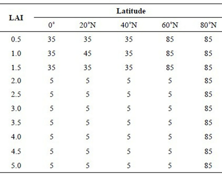
Table 1. Simulated leaf inclination angles in degrees for latitude bands on the summer solstice (solar declination 23.5˚). Each column contains the leaf inclination angles with increasing depth in the canopy for a given latitude. The LAI column is the cumulative LAI from the top of the canopy. The leaf inclination angles vary between 5˚ for horizontal leaves to 85˚ for vertical leaves.
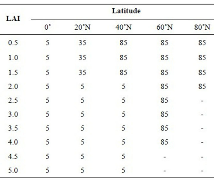
Table 2. Simulated leaf inclination angles in degrees for latitude bands on the equinox (solar declination 0˚). Each column contains the leaf inclination angles with increasing depth in the canopy for a given latitude. The LAI column is the cumulative LAI from the top of the canopy. The leaf inclination angles vary between 5˚ for horizontal leaves to 85˚ for vertical leaves. Table entries containing a dash (-) have APAR levels in that layer that were less than the light compensation point.
the LAD pattern is similar to the summer’s LAD. However, 40˚N the distribution changes from the tropical pattern of mostly horizontal leaves to a more boreal pattern of erect leaves at the top of the canopy. North of 60˚ N the entire canopy consists of vertical leaves.
A sensitivity analysis was performed to evaluate the effects of variations to the initial simulations. Initially, the canopy model contained only leaves, and a second model run added branches to the canopy. Since branches contain non-photosynthetic material, the model was restructured into pairs of layers, where each layer pair had an upper layer of leaves and a lower layer of branches. Branch area was taken to be a tenth of the leaf area, or 0.05 per layer. These simulations result in the same leaf angle structure as the leaf only simulations described above, although the branches intercept between three to seven percent of the PAR.
Changes in solar zenith angle throughout the day are a driver for leaf angles in this model, so another variation of the simulations involves altering the fraction of incident diffuse, i.e. nondirectional, light. If the proportion of diffuse light in the incoming radiation is increased, two effects are observed in the leaf angle distributions. First, the top layers of the tropical canopies become more erect. For example, with 60% incoming diffuse light, the top layer leaf angle at 40˚N in summer changes from 35˚ to 55˚. The second effect is that leaves begin to become horizontal higher in the canopy. Increasing the proportion of diffuse radiation for the boreal canopies has no effect on their leaf angle distribution.
The addition of perturbations to the original simulations in the form of additional canopy components by including branches and increasing the fraction of nondirectional diffuse light were found to have little effect on the general patterns of LAD suggesting some robustness to the model results.
The simulated LAD patterns can be evaluated through comparison with measured LAD profiles. It is difficult and time consuming to measure leaf angles in forests; however, some studies have measured leaf angles along with depth in the canopy. Hutchison et al. [23] measured the architecture of a mature deciduous forest near Oak Ridge, Tennessee at approximately 36˚N. The forest consisted of Quercus alba L., Q. prinus L., Q. velutina Lam., Q. falcata Michx., Acer rubrum L. and Liriodendron tulipifera L. Measurements of leaf inclinations were made with a protractor and plumb line. At the top of the canopy the leaf inclination was found to be approximately 50˚ and remained near that value within the main canopy. In the understory the leaf angle dropped down to near 15˚. This pattern is similar to the model results, particularly if one assumes a fair proportion of the incoming light is diffuse in East Tennessee.
Another study of canopy architecture was made by Miller and Lin [22] for a stand of Acer rubrum L. in Coventry, Connecticut at approximately 42˚N. They used a point drop method; at each sample point a weighted line was dropped from above the canopy and every leaf touched by the line was measured. They report that the leaves at the top of the canopy have a wide distribution of leaf angles. In the upper canopy the probability of encountering any given leaf angle between 15˚ and 75˚ is approximately 0.2. The point drop method may underestimate the fraction of erect leaves. Since erect leaves have a small horizontal cross section, they are less likely to be intercepted by the vertical sample. The leaf angles in the lower canopy were found to be within 15˚ of horizontal with a probability of 0.7.
Ford and Newbould [21] measured leaf angles in a coppiced woodland of sweet chestnut (Castanea sativa Mill.) near Kent in the United Kingdom at approximately 51˚N. They found mean leaf inclination angles at the canopy top to be about 36˚. The inclination angles dropped to 15˚ when the cumulative LAI from the top of the canopy was 5. The upper canopy leaf angles match the model results for the summer case at 40˚N; however, the model indicates that the transition to horizontal leaves should occur higher in the canopy than these measurements show.
In the Craigieburn Range, South Island, New Zealand, Hollinger [24] measured leaf inclination angles of the evergreen mountain beech (Nothofagus solandri Hook.f.). The site was located at 43˚08'S. Mean leaf inclination angles were 43.3˚ for the canopy top, 22.1˚ for the midcanopy, and 17.0˚ for the lower canopy. The vertical distributions of leaf angle for a 46-year-old stand of Japanese cypress (Chamaecyparis obtusa Endl.) in central Japan decreased exponentially from top to bottom of the canopy, ranging in value from greater than 55˚ to 30.3˚ [35]. Again, these studies show a general pattern similar to the simulated summer case at 40˚N.
These measurements of the vertical patterns leaf angles within forest canopies do not verify the results of the simulations. However, they show similar patterns to the simulated LAD and show leaf angles varying with depth in the canopy.
Using the leaf angle distributions predicted for each latitude, the SAIL model calculates the canopy reflectance in the visible and near-infrared bands and these values are used to determine NDVI. The model also calculates total daily fAPAR as it varies with increasing LAI, allowing an analysis of the relationship between canopy structure, fAPAR, and NDVI as they vary over space and time.
Figures 2(a) and (b) show how daily fAPAR varies with LAI for five latitudes on the summer solstice (solar declination 23.5˚) and the equinox (solar declination 0˚). LAI was varied by adding layers to the canopy with the leaf angles predicted as described above, so this plot can also be interpreted as a measure of cumulative fAPAR with depth in the canopy. In all cases, the fAPAR curves vary smoothly with LAI. The curves for 0˚ through 60˚N on the summer solstice and 0˚ through 40˚N on the equinox are nearly identical and saturate at about the same value, approximately 97%. The effect of varying solar zenith angles appears at higher latitudes. The curve for 80˚N on the summer solstice is the same as the curve for 60˚N on the equinox. The very low sun angles at 80˚N on the equinox result in a very high percentage of fAPAR even with low LAI.
The relationships between LAI and NDVI at 10:00 A.M. solar time (Figures 3(a) and (b)) are more variable than the relationships between LAI and fAPAR. There are different curvatures for most lines, the saturation points vary for most curves and there are discontinuities in some curves. In the plots for the summer solstice (Figure 3(a)) the latitudes between 0˚N and 40˚N have canopies with the tropical leaf angle distributions and show identical relationships between NDVI and LAI. At 60˚N the relationship shows a discontinuity when the canopy reaches a layer where the more erect leaves change to horizontal leaves at a LAI of 2. The line for the 80˚N boreal canopy has its own track, having much lower NDVI values than the tropical canopies at low LAI. On the equinox (Figure 3(b)), the relationships for every latitude has its own distinct curve. The curves for 0˚N and 20˚N are nearly the same as on the solstice but they are no longer identical. The curve for 40˚N is nearly the
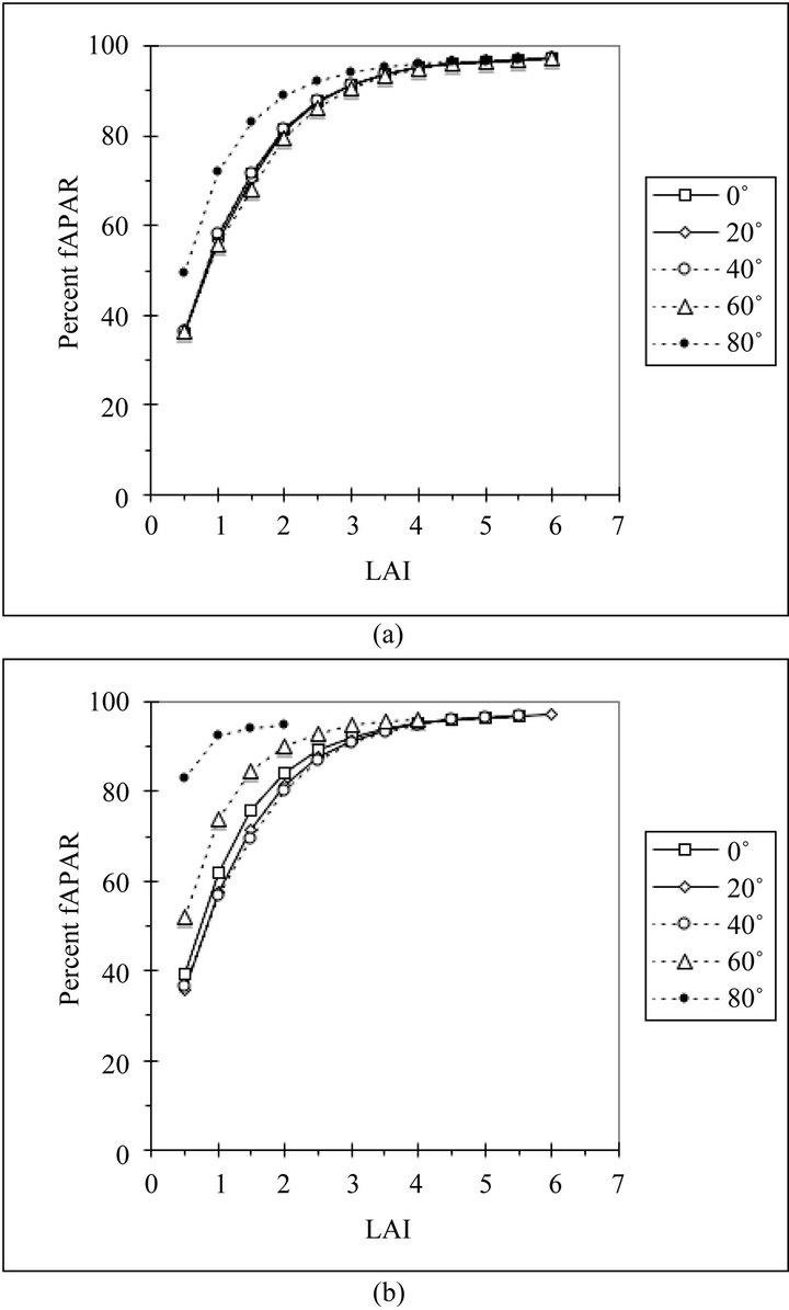
Figure 2. (a) Relationship between canopy LAI and daily fAPAR for canopies predicted by the model at five northern latitudes on the summer solstice (solar declination 23.5˚); (b) Relationship between canopy LAI and daily fAPAR for canopies predicted by the model at five northern latitudes on the equinox (solar declination 0˚).
same as the 60˚N curve on the solstice, showing the same discontinuity at a LAI of 2. The 60˚N curve for the equinox is similar to the 80˚N curve on the solstice. The 80˚N curve for the equinox has the highest values of NDVI.
The relationship between NDVI and fAPAR produces three distinct curves depending on canopy type (Figures 4(a) and 4(b)). The tropical canopies, 0˚ through 40˚N on the solstice and 0˚N and 20˚N on the equinox, have an upward curvature. While the boreal canopies, 80˚N on the solstice and 60˚N and 80˚N on the equinox, have a downward curvature. The canopies at 60˚N on the solstice and 40˚N on the equinox begin with the boreal curves and make a transition to the tropical curves at higher values of canopy LAI. Figures 4(a) and (b) show how attempting to predict percent fAPAR from NDVI may result in errors of as much as 40%, if one does
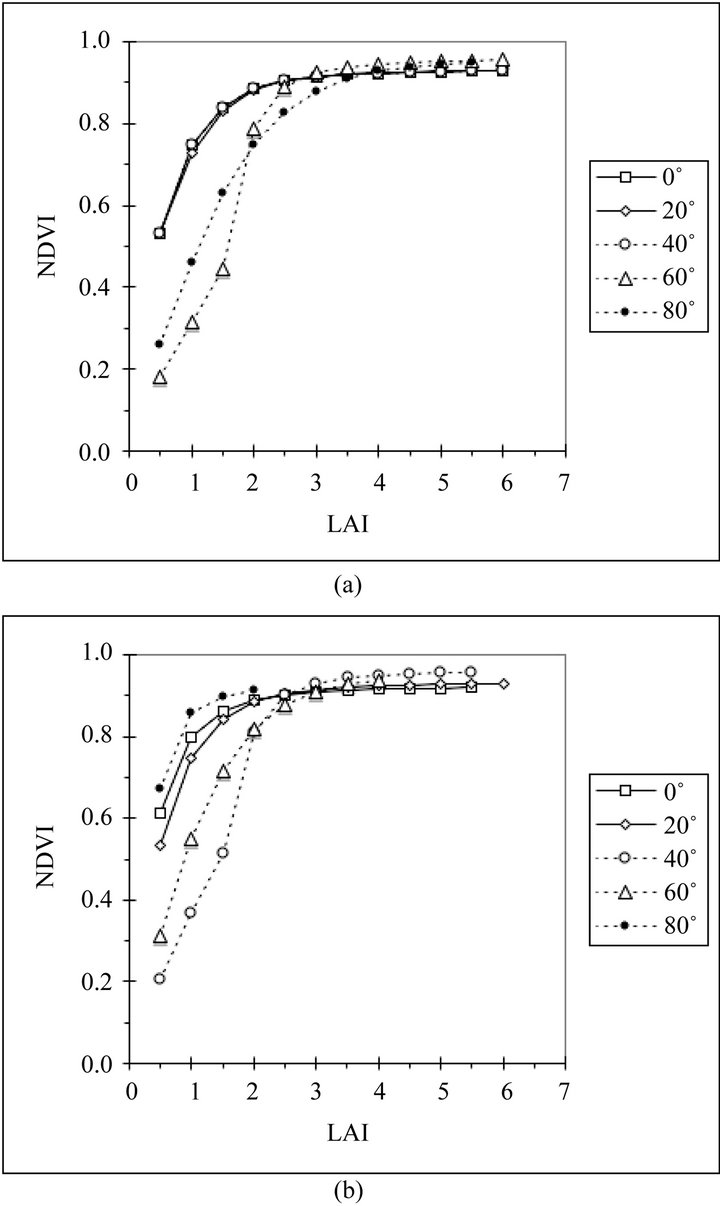
Figure 3. (a) Relationship between canopy LAI and nadir view NDVI at 10 AM solar time for canopies predicted by the model at five northern latitudes on the summer solstice (solar declination 23.5˚); (b) Relationship between canopy LAI and nadir view NDVI at 10 AM solar time for canopies predicted by the model at five northern latitudes on the equinox (solar declination 0˚).
not take into account the effects of canopy structure and latitude.
The variation of leaf angle with depth in the canopy may also affect other approaches to remote sensing of vegetation. For example, lidars can directly measure the vertical distributions of intercepted surfaces in a canopy, and from that infer the distribution of leaf area [36]. The conversion between the area intercepted by the vertical beam and leaf area depends on leaf inclination angles. Figure 5 shows the expected interception of a vertical beam by layers of a canopy for the 40˚N case. In this example, each layer has the same LAI, but there is a significant difference in the interception with depth in the canopy due to variations in leaf inclination angles alone. Seasonal and spatial variations in leaf angles as shown in
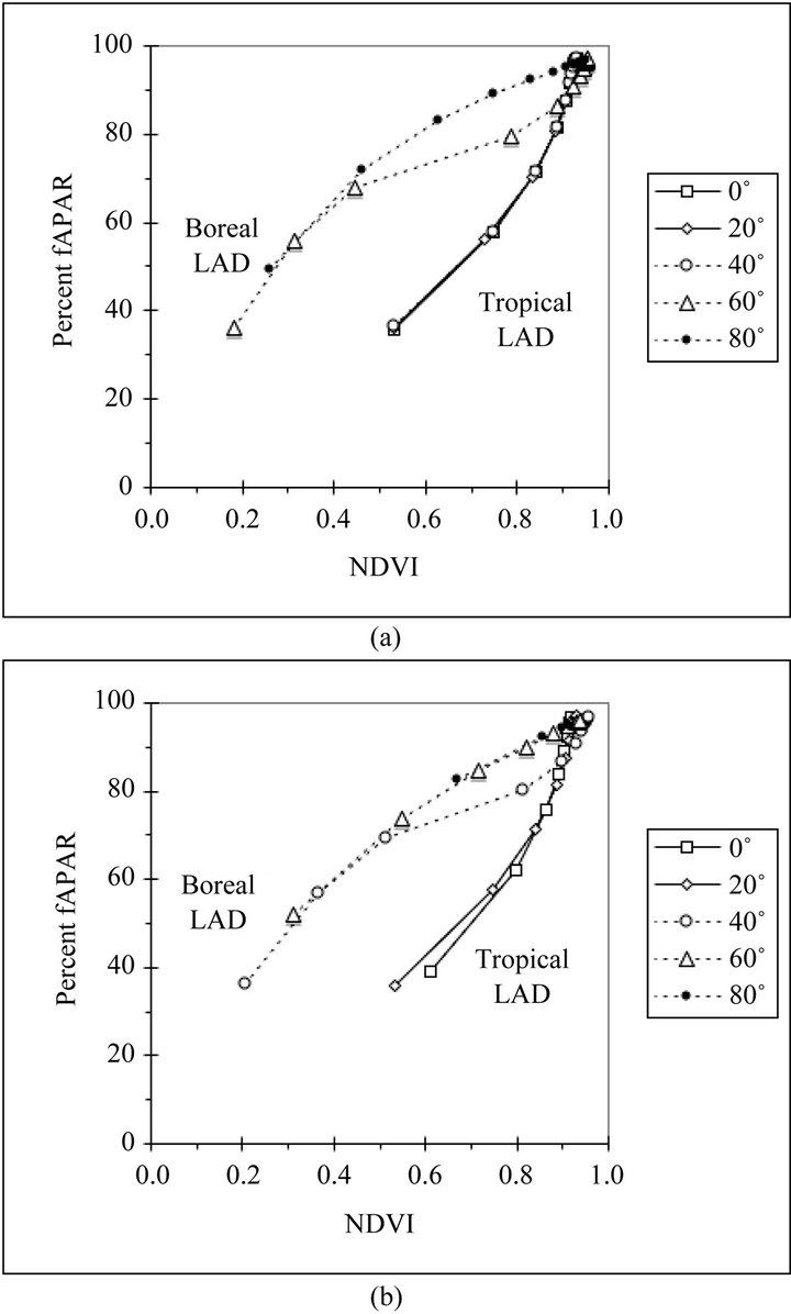
Figure 4. (a) Relationship between nadir view NDVI at 10 AM solar time and daily fAPAR for canopies predicted by the model at five northern latitudes on the summer solstice (solar declination 23.5˚); (b) Relationship between nadir view NDVI at 10 AM solar time and daily fAPAR for canopies predicted by the model at five northern latitudes on the equinox (solar declination 0˚).
these simulations can result in significant differences in the interception of the layers that must be accounted for when processing lidar data to accurately describe the vertical distribution of leaf area.
4. Conclusions
This simulation exercise suggests that there may be global patterns of LADs in vegetation canopies. For canopies optimizing photosynthesis within each layer, the LADs are driven by location and sun angle resulting in latitudinal and seasonal patterns of canopy structure. The optimal LAD for tropical regions has leaves in the upper canopy that are around 35˚ and horizontal in the lower canopy. In the high latitudes, the optimal canopy LAD consists entirely of vertical leaves. In the mid-lati-
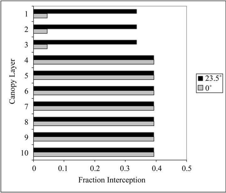
Figure 5. The fraction of a vertical beam intercepted by each canopy layer for the 40˚N case on the solstice with solar declination 23.5˚ (black bars), and the equinox with 0˚ declination (gray bars). For the canopy layers, 1 is the topmost layer, and each layer has an LAI of 0.5.
tudes, the optimal LAD changes with season, blending these two patterns. There are too few measurements of LAD, particularly of tropical and boreal canopies, to allow a verification of the model results.
The model results further indicate that spatial and temporal variation of LAD complicates the interpretation of remotely sensed data. The simulations indicate relationships between NDVI and fAPAR are nonlinear with curvature changes depending on LAD and location. The tropical and boreal LADs each produce a distinct NDVI - fAPAR relationship. Significant errors in estimation of fAPAR may occur by not taking into account spatial variability in LAD. In the middle latitudes errors in fAPAR estimation from NDVI may also occur if seasonal changes in LAD are not taken into account. LAD patterns are an important, but little understood, factor in the analysis of global remote sensing observations.
This simple modeling “thought experiment” produced interesting results, pointing to the need for further work using models with more complex 3-dimensional descriptions of vegetation canopies along with measurements of leaf angles with depth in canopies.
5. Acknowledgements
The author thanks Richard Waring for his many useful comments.
REFERENCES
- P. G. Jarvis and J. W. Leverenz, “Productivity of Temperate, Deciduous and Evergreen Forests,” In: O. L. Lange, C. B. Osmond and H. Ziegler, Eds., Physiological Plant Ecology IV, Springer-Verlag, New York, 1983, pp. 233- 280. doi:10.1007/978-3-642-68156-1_9
- D. A. King, “The Functional Significance of Leaf Angle in Eucalyptus,” Australian Journal of Botany, Vol. 45, No. 4, 1997, pp. 619-639. doi:10.1071/BT96063
- I. Cowan, “Regulation of Water Use in Relation to Carbon Gain in Higher Plants,” In: O. L. Lange, P. S. Nobel, C. B. Osmond and H. Ziegler, Eds., Physiological Plant Ecology II. Water Relations and Carbon Assimilation, Encyclopaedia of Plant Physiology Vol. 12B, Springer, Berlin, 1981, pp. 589-614.
- F. Baret and G. Guyot, “Potential and Limits of Vegetation Indices for LAI and APAR Assessment,” Remote Sensing of Environment, Vol. 35, No. 2-3, 1991, pp. 161- 173. doi:10.1016/0034-4257(91)90009-U
- S. N. Goward and K. F. Huemmrich, “Vegetation Canopy PAR Absorptance and the Normalized Difference Vegetation Index: An Assessment Using the SAIL Model,” Remote Sensing of Environment, Vol. 39, No. 2, 1992, pp. 119-140. doi:10.1016/0034-4257(92)90131-3
- J. Ehleringer and K. S. Werk, “Modifications of Solar Radiation Absorption Patterns and Implications for Carbon Gain at the Leaf Level,” In: T. Givnish, Ed., On the Economy of Plant Form and Function, Cambridge University Press, Cambridge, 1986, pp. 57-82.
- E. Ezcurra, C. Montana and S. Arizaga, “Architecture Light Interception and Distribution of Larrea-spp in the Monte Desert Argentina,” Ecology, Vol. 72, No. 1, 1991, pp. 23-34. doi:10.2307/1938899
- J. Ross, “The Radiation Regime and Architecture of Plant Stands,” Dr. W. Junk, The Hague, 1981. doi:10.1007/978-94-009-8647-3
- N. S. Goel and D. E. Strebel, “Simple Beta Distribution Representation of Leaf Orientation in Vegetation Canopies,” Agronomy Journal, Vol. 76, No. 5, 1984, pp. 800- 802. doi:10.2134/agronj1984.00021962007600050021x
- D. D. Baldocchi, B. A. Hutchison, D. R. Matt and R. T. McMillen, “Canopy Radiative Transfer Models for Spherical and Known Leaf Inclination Angle Distributions: A Test in an Oak-Hickory Forest,” Journal of Applied Ecology, Vol. 22, No. 2, 1985, pp. 539-556. doi:10.2307/2403184
- H. Barclay, “Distribution of Leaf Orientations in Six Conifer Species,” Canadian Journal of Botany, Vol. 79, No. 4, 2001, pp. 389-397. doi:10.1139/b01-014
- W. K. Smith, D. T. Bell and K. A. Shepherd, “Associations between Leaf Structure, Orientation, and Sunlight Exposure in Five Western Australian Communities,” American Journal of Botany, Vol. 85, No. 1, 1998, pp. 56-63. doi:10.2307/2446554
- W. K. Smith, T. C. Vogelmann, E. H. Delucia, D. T. Bell and K. A. Shepherd, “Leaf Form and Photosynthesis,” Bioscience, Vol. 47, No. 11, 1997, pp. 785-793. doi:10.2307/1313100
- C. Werner, R. J. Ryel, O. Correia and W. Beyschlag, “Structural and Functional Variability within the Canopy and its Relevance for Carbon Gain and Stress Avoidance,” Acta Oecologica, Vol. 22, No. 2, 2001, pp. 129- 138. doi:10.1016/S1146-609X(01)01106-7
- J. Ehleringer and I. Forseth, “Solar Tracking by Plants,” Science, Vol. 210, No. 4474, 1980, pp. 1094-1098. doi:10.1126/science.210.4474.1094
- D. S. Kimes and J. A. Kircher, “Diurnal Variations of Vegetation Canopy Structure,” International Journal of Remote Sensing, Vol. 4, No. 2, 1983, pp. 257-271. doi:10.1080/01431168308948545
- J. L. Monteith, “Light Distribution and Photosynthesis in Field Crops,” Annals of Botany, Vol. 29, No. 113, 1965, pp. 17-37.
- H. Horn, “The Adaptive Geometry of Trees,” Princeton University Press, Princeton, 1971.
- D.S. Falster and M. Westoby, “Leaf Size and Angle Vary Widely Across Species: What Consequences for Light Interception?” New Phytologist, Vol. 158, No. 3, 2003, pp. 509-525. doi:10.1046/j.1469-8137.2003.00765.x
- W. G. Duncan, “Leaf Angles, Leaf Area, and Canopy Photosynthesis,” Crop Science, Vol. 11, No. 4, 1971, pp. 482-485. doi:10.2135/cropsci1971.0011183X001100040006x
- E. D. Ford and P. J. Newbould, “The Leaf Canopy of a Coppiced Deciduous Woodland. I. Development and Structure,” Journal of Ecology, Vol. 59, No. 3, 1971, pp. 843-862. doi:10.2307/2258144
- D. R. Miller and J. D. Lin, “Canopy Architecture of a Red Maple Edge Stand Measured by a Point Drop Method,” In: B. A. Hutchison and B. B. Hicks, Eds., The Forest-Atmosphere Interaction, D. Reidel, Boston, 1985, pp. 59-70. doi:10.1007/978-94-009-5305-5_4
- B. Hutchison, D. Matt, R. McMillen, L. Gross, S. Tajchman and J. Norman, “The Architecture of Deciduous Forest Canopy in Eastern Tennessee, USA,” Journal of Ecology, Vol. 74, No. 3, 1986, pp. 635-646. doi:10.2307/2260387
- D. Y. Hollinger, “Canopy Organization and Foliage Photosynthetic Capacity in a Broad-Leaved Evergreen Montane Forest,” Functional Ecology, Vol. 3, No. 1, 1989, pp. 53-62. doi:10.2307/2389675
- T. J. Herbert, “Leaf Inclination of Dryas octopetala L. and its Dependence on Latitude,” Polar Biology, Vol. 13, No. 2, 1993, pp. 141-143. doi:10.1007/BF00238547
- D. S. Bartlett, M. A. Hardisky, R. W. Johnson, M. F. Gross, V. Klemas and J. M. Hartman, “Continental Scale Variability in Vegetation Reflectance and its Relationship to Canopy Morphology,” International Journal of Remote Sensing, Vol. 9, No. 7, 1988, pp. 1223-1241. doi:10.1080/01431168808954930
- P. J. Sellers, “Canopy Reflectance, Photosynthesis and Transpiration,” International Journal of Remote Sensing, Vol. 6, No. 8, 1985, pp. 1335-1372. doi:10.1080/01431168508948283
- B. J. Choudhury, “Relationships between Vegetation Indices, Radiation Absorption and Net Photosynthesis Evaluated by a Sensitivity Analysis,” Remote Sensing of Environment, Vol. 22, No. 2, 1987, pp. 209-234. doi:10.1016/0034-4257(87)90059-9
- L. Alexander, “SAIL Canopy Model Fortran Software,” NASA Johnson Space Center, Houston, 1983.
- W. Verhoef, “Light Scattering by Leaf Layers with Application to Canopy Reflectance Modeling: The SAIL Model,” Remote Sensing of Environment, Vol. 16, No. 2, 1984, pp. 125-141. doi:10.1016/0034-4257(84)90057-9
- L. E. Hipps, G. Asrar and E. Kanemasu, “Assessing the Interception of Photosynthetically Active Radiation in Winter Wheat,” Agricultural Meteorology, Vol. 28, No. 3, 1983, pp. 253-259. doi:10.1016/0002-1571(83)90030-4
- W. D. Sellers, “Physical Climatology,” University of Chicago Press, Chicago, 1965.
- S. N. Goward, C. J. Tucker and D. G. Dye, “North American Vegetation Patterns Observed with the NOAA- 7 Advanced Very High Resolution Radiometer,” Vegetatio, Vol. 64, No. 1, 1985, pp. 3-14. doi:10.1007/BF00033449
- C. O. Justice, J. R. G. Townshend, B. N. Holben and C. J. Tucker, “Analysis of the Phenology of Global Vegetation using Meteorological Satellite Data,” International Journal of Remote Sensing, Vol. 6, No. 8, 1985, pp. 1271- 1318. doi:10.1080/01431168508948281
- H. Utsugi, M. Araki, T. Kawasaki and M. Ishizuka, “Vertical Distributions of Leaf Area and Inclination Angle, and their Relationship in a 46-Year-Old Chamaecyparis obtusa Stand,” Forest Ecology and Management, Vol. 225, No. 1-3, 2006, pp. 104-112. doi:10.1016/j.foreco.2005.12.028
- R. O. Dubayah and J. B. Drake, “Lidar Remote Sensing for Forestry,” Journal of Forestry, Vol. 98, No. 6, 2000, pp. 44-46.