The Stability of a Rotating Cartesian Plume in the Presence of Vertical Boundaries

doi:10.4236/ojfd.2014.42016

Open Journal of Fluid Dynamics
Vol.4 No.2(2014), Article ID:46732,19 pages DOI:10.4236/ojfd.2014.42016

Khaled S. Al-Mashrafi¹, Ibrahim A. Eltayeb²

●Abstract

●Full-Text PDF

●Full-Text HTML

●Full-Text ePUB

●Linked References

●How to Cite this Article

¹Section of Applied Sciences, Department of Human Resources Development, General Directorate of Education in Eastern Region, Ministry of Education, Sur, Oman

²Department of Mathematics and Statistics, College of Science, Sultan Qaboos University, Muscat, Oman

Email: P001175@student.squ.edu.om

This work is licensed under the Creative Commons Attribution International License (CC BY).

http://creativecommons.org/licenses/by/4.0/

Received 15 April 2014; revised 15 May 2014; accepted 22 May 2014

ABSTRACT

The effect of two fixed vertical boundaries, a finite distance apart, on the dynamics of a column of buoyant fluid rising in a less buoyant fluid is investigated in the presence of vertical rotation. It is shown that the presence of the boundaries introduces two main effects on a rotating plume. They tend to stabilise the plume but succeed only reducing the value of the growth rate and the plume remains unstable for all finite values of the distance between the boundaries and the plume. In the absence of the sidewalls, two modes of the instability were found known as the sinuous mode and the varicose mode. The influence of the boundaries is such that it reduces the growth rate of the varicose mode more than that of the sinuous mode and consequently the modified sinuous mode is always preferred in the presence of the boundaries.

Keywords:Compositional Plumes, Stability, Growth Rate, Bounded Domain, Rotation

1. Introduction

The study of the dynamics of compositional plumes is important for many real life applications in industry ([1] - [6] ), geophysics ([7] -[25] ) and environment ([26] -[34] ). While the presence of the compositional plumes can be harmful (e.g., in iron bars), it is useful in geophysics (e.g., the hot compositional plumes, that rise from the inner core boundary of the Earth into the outer core interact with the rotation and magnetic field of the Earth and may contribute to the Geodynamo). Such a wide range of applications has motivated many studies on various aspects of the dynamics of compositional plumes. These studies are experimental and theoretical. The experimental works on the dynamics of compositional plumes observed that the plume flow seems to be stable (Sample and Hellawell [35] ; Chen and Chen [36] ; Hellawell et al. [37] ). The laboratory studies by Hellawell et al. [37] find that the plumes are thin and long, and its top part tends to break up and disappears. Classen et al. [38] experimentally studied the dynamics of compositional plumes under the influence of vertical rotation to find that the plumes are unstable and break into blobs. On the other hand, the theoretical works on the stability of the plumes showed that the Cartesian plume is always unstable in the absence of rotation (Eltayeb and Loper [16] ) and in the presence of rotation (Eltayeb and Hamza [18] ). These studies assumed that the plume rises vertically in a fluid of unbounded domains. While the experimental studies were conducted in bounded regions to show that the plume was stable, the theoretical models were conducted in unbounded domains to find that the plume was unstable. Thus it is of interest to examine the influence of the vertical boundaries on the dynamics of the plumes. The mathematical model by Al Mashrafi and Eltayeb [6] investigated the influence of the two fixed vertical boundaries on the dynamics of the plumes. They tested the stability of non-rotating Cartesian plumes in a bounded domain to find that the presence of two vertical boundaries affects the stability, but the plumes remain unstable. Moreover, they found that the plume was stable when it was close to the boundary but had a large thickness and the material diffusion is potent in the thin layer between the plume and the nearest boundary.

Motivated by real life applications and laboratory results, we study here the influence of vertical rotation on the dynamics of bounded Cartesian plume. In general, the purpose of this study is to extend the theoretical model by Al Mashrafi and Eltayeb [6] on the dynamics of a Cartesian compositional plume in bounded regions to include the action of vertical rotation. The model by Al Mashrafi and Eltayeb [6] consisted of a column of buoyant fluid of finite thickness, , rising vertically in another less buoyant fluid bounded by two fixed vertical walls located at and. The system was infinite in the and directions. In the current study, we consider that the whole system rotates about the vertical with a uniform angular speed, (see Figure 1).

In Section 2, we formulate the model mathematically and state the boundary conditions of the system. The presence of rotation introduces an additional parameter, , which is a measure of the Coriolis force relative to the viscous force, and this parameter referred to hereinafter as the rotation parameter, defined by

(1)

where is the Taylor number, is the kinematic viscosity and is the unit of length (see Equation (6) below). In Section 3, we investigate the influence of the vertical boundaries on the linear stability of a rotating

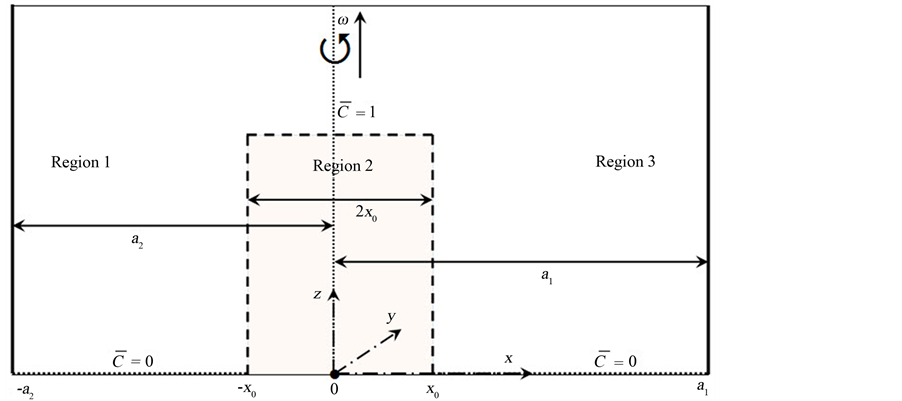
Figure 1. The geometry of the problem showing the profile of the basic state concentration of light material, , representing a plume of width, , and concentration, 1 , rising vertically in a finite fluid of width, , and concentration, 0. The system rotates uniformly about the vertical with angular speed,. The plume divided the system into three regions: region 2 represents the plume whereas regions 1 and 3 represent the surrounding fluid.

bounded Cartesian plume. The problem of the rotating plume was studied by Eltayeb and Hamza [18] in the absence of boundaries. In Section 4, we discuss the effect of the boundaries on the stability of a rotating plume. The growth rate is maximised over the wave numbers plane in the parameter space. In Section 5, we make some concluding remarks.

2. Formulation of the Problem

We consider a two-component fluid, in which the concentration of the solvent component (light material) is and the temperature is, rotating uniformly about the vertical with angular velocity. The fluid has kinematic viscosity, , and thermal diffusivity, , and material diffusion is negligible. The dimensionless equations of the system have been derived by Eltayeb and Hamza [18] . They are

(2)

(3)

(4)

(5)

Here R, and are the Grashoff number, the Prandtl number and the rotation parameter, respectively, defined by

(6)

where is the Taylor number and, and are characteristic units of velocity, length and concentration, respectively (Al Mashrafi and Eltayeb [6] ), and, , , , , , , , are the velocity vector, the pressure, the constant gravitational acceleration, the upward unit vector, the time, the thermal expansion coefficient, the compositional expansion coefficient, the density, the uniform temperature gradient and the subscript “” in the Equation (2) refers to reference values.

We consider a basic concentration profile

(7)

which defines a plume of thickness, , rising with velocity in the presence of mean temperature and mean pressure such that

(8)

(9)

which are the same equations obtained in the absence of rotation. The presence of rotation does not affect the basic state, and the solution of (8) and (9) is the same as in the absence of rotation. We include it here for easy reference:

(10)

where, and are defined by

(11)

3. The Stability Analysis

In this section, we use the perturbation Equations (14)-(17) to investigate the linear stability of the basic state solution given by (10). We assume that the interface at the plane is given a small harmonic disturbance of the form

(12)

where and are the wavenumber components in the plane, is the growth rate and refers to the complex conjugate.

The disturbance (12) will propagate into the fluid, and affect the second interface and the variables of the system to produce the perturbations. Consequently, the interface at can be written in the form

(13)

where is a measure of the amplitude of the interface and it is evaluated as a part of the solution. The perturbations introduced into the system are governed by the dimensionless equations (see Al Mashrafi and Eltayeb [6] )

(14)

(15)

(16)

(17)

where, , and are the perturbations in velocity, pressure, temperature and concentration, respectively.

The perturbation variables take the form

(18)

in which the factors, , and are introduced in the variables, and, respectively, for convenience.

Substituting the variables (18) into the Equations (14)-(17) and after some arrangements we get the following equations

(19)

(20)

(21)

(22)

(23)

(24)

(25)

subject to the boundary conditions

(26)

(27)

(28)

(29)

where the variable is related to the vertical component of vorticity and is defined as

(30)

and we have introduced the notation

(31)

(cf. Al Mashrafi and Eltayeb [6] ).

We use the same method adopted in Al Mashrafi and Eltayeb [6] and expand the perturbation variables and the growth rate in the small parameter, thus

(32)

where indicates any of the perturbation variables, , , , and.

It turned out that the leading order terms in the equations determines the stability of the system. The relevant equations and the boundary conditions are then obtained from (19)-(24) and (26)-(29) by neglecting the terms with. In order to facilitate comparison with the results of the non-rotating case, we shall maintain the subscript 0. The equations are given by

(33)

(34)

(35)

(36)

(37)

(38)

The associated boundary conditions are obtained from (26)-(29) by introducing the subscript 0 to all the variables and the subscript 1 to.

The system (33)-(38) together with the boundary conditions poses an eigenvalue problem for the growth rate, , which determines the stability of the system. The real part governs the variations of the amplitude of the disturbance with time, and hence it determines the stability of the disturbance. If it is negative for all possible values of the wavenumbers and, then the plume is stable, while if at least one pair of and gives a positive value, then the plume is unstable. If vanishes for all values of the wavenumbers, the plume is neutrally stable. If the preferred mode occurs for, both non-zero, it is referred to as a 3-dimensional mode (oblique), and if, it is called 2-dimensional (vertical). The case and is found not to occur. The imaginary part determines the phase speed of the disturbance. The vertical phase speed and the horizontal phase speed are defined as

(39)

We note that is defined only if.

We operate on Equation (33) with, and use Equations (34)-(36) to get

(40)

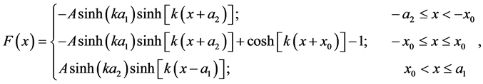
The general solution of the differential Equation (40) can be written in the form

(41)

where the superscript refers to the three regions of the system (see Figure 1), , are constants, and are the roots of the cubic equation

(42)

with is given by

(43)

We use the Equations (34)-(36) and the solution (41) to obtain

(44)

The Equation (37) can be solved in the form a complementary function and particular solution to find

(45)

where, are constants, and, are given by

(46)

Now we apply the boundary conditions at, , and solve the resulting algebraic equations for the constants, , , for The details of the solution are given in the Appendix A.

The growth rate is given by the quadratic equation

(47)

where and are given in the Appendix A.

Solving Equation (47) yields

(48)

and the displacement is given by

(49)

in which and are defined in the Appendix A.

We note that, as in the absence of rotation, the system has two modes. The upper sign in the expression (48) corresponds to the modified varicose mode (MV) and the lower sign refers to the modified sinuous mode (MS).

4. Discussions of the Results

The growth rate (48) is evaluated numerically in the plane as a function of the parameters, , and for both modes. The contours of in the plane are plotted for sample values of the parameters, , and in the Figures 2-4.

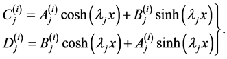
In Figure 2, we present a comparison between the contours of the two modes MV and MS for different values of the Taylor number, , when, and. We note that the MV mode always possesses a minimum with negative growth rate and one or two maxima with positive growth rates while the MS mode has

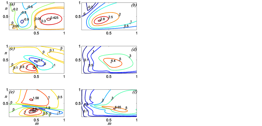
Figure 2. Contours of the growth rate , , of the modes MV, as in (a), (c), (e) and MS, as in (b), (d), (f) for the rotating bounded Cartesian plume where, ,. Here for (a), (b); for (c), (d); and for (e), (f). Note that the preferred mode is MS.

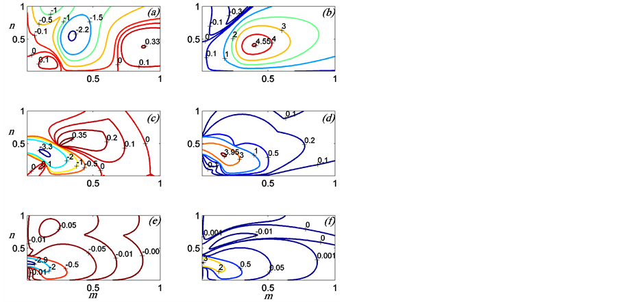
Figure 3. Contours of the growth rate, , of the modes MV, as in (a), (c), (e) and MS, as in (b), (d), (f) for, ,. Here for (a), (b); for (c), (d); and for (e), (f). Note that the preferred mode of the instability is 2-dimensional when.

a minimum with negative growth rate only when is small and one maximum with positive growth rate which is larger than that of the corresponding MV mode. This indicates that the MS mode is preferred for this set of parameters. The local maxima correspond to 3-dimensional modes and the largest maximum always increases with the increase in the rotation parameter.

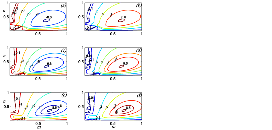
Figure 4. Isolines of the growth rate , , as in (a), (c), (e) and as in (b), (d), (f) for, ,. Here for (a), (b); for (c), (d); and for (e), (f). Note that at fixed point, the values of and are nearly same but there different in the sign.

Figure 3 presents the influence of the distance between the plume and the nearest sidewall on the stability of the plume when the thickness of the plume and the rotation parameter are held fixed at and. The figure is plotted for three different values of: for subfigures (a), (b); for subfigures (c), (d); and for subfigures (e), (f). When the plume is situated half-way between the sidewalls, the MV mode has a negative growth rate everywhere and hence stable while the MS mode has a growth rate that is positive everywhere and hence is preferred. The local maximum possesses a vanishing horizontal wave number and hence propagates vertically. As the plume moves towards a wall, the growth rates of both modes increase and the MV mode develops local maxima with positive growth rates but they are not preferred because the MS mode local maximum increases as well and becomes 3-dimenaional.

Figure 4 illustrates the influence of the plume thickness on the contours of the growth rate for fixed values of the rotation parameter and the distance between the two sidewalls when the plume is situated half-way between the two sidewalls. As increases from, the growth rate for MS mode, which is positive everywhere, increases and that of the MV mode, which is negative everywhere, decreases until reaches a critical value, , when the growth rate of the MS mode decreases and that of the MV mode increases.

The contours of Figures 2-4 indicate that the preferred mode of instability is the modified sinuous (MS) mode. This indication is quantified by calculating the maximum growth rate and the associated wave numbers and phase speeds for different values of the parameters. For fixed values of, , and, we maximize over the wave numbers and by demanding that

(50)

The solution of (50) gives the values and at maximum growth rate, , calculated from (48) for these values of and to give, together with the corresponding value of the phase speed, the parameters of the preferred mode. For fixed parameters, , and, and particular mode, all possible local maxima of are identified and the largest value taken together with the corresponding wavenumbers and phase speeds as defining the preferred mode for that set of parameters for that mode. This is carried out for both modified varicose (MV) and modified sinuous (MS) modes, and the largest is chosen as the preferred mode. A sample of the results is given in Figures 5-9.

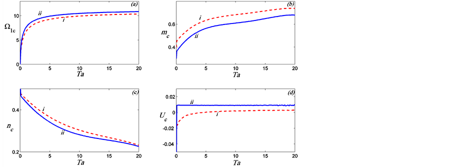
Figure 5. The preferred mode parameters are plotted in (a), (b), (c), (d) as a function of , for, and two different values of and the plume half-way between the sidewalls. The roman numbers and refer to and, respectively.

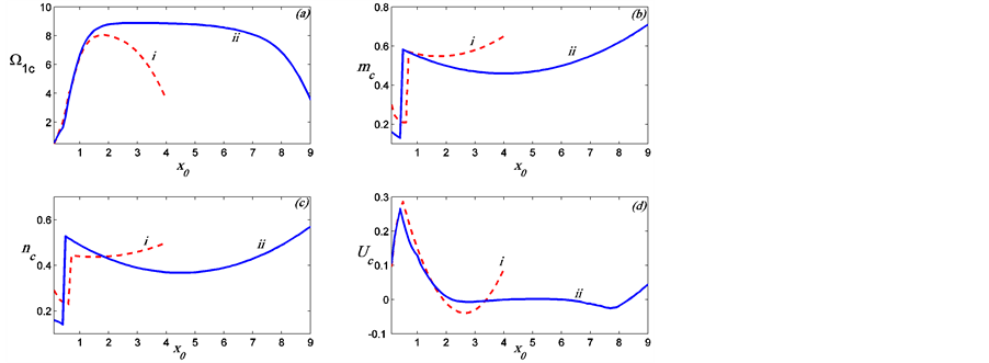
Figure 6. The preferred mode parameters are plotted in (a), (b), (c), (d) as a function of, for, and two different values of and the plume half-way between the sidewalls. The roman numbers and refer to and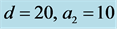, respectively.

Figure 5 and Figure 6 illustrate the influence of the distance between the boundaries on the preferred mode of instability of the rotating plume. In Figure 5, the preferred mode parameters are plotted as a function of for fixed and two values of the distance between the sidewalls, , for a plume situated half-way between the sidewalls. It is found that the preferred mode is the MS mode and the influence of the boundaries tends to stabilise the plume but only reduces the growth rate slightly. The horizontal and vertical wavenumbers are increased while the phase speeds are reduced as the distance, , between the two walls is reduced.

Figure 6 presents the preferred mode of instability as a function of and fixed where the plume is equidistant from the two walls and takes the values 10 and 20. The growth rate increases rapidly as increases from zero until it reaches a maximum when the plume occupies the middle half of the region between the sidewalls. As the thickness of the plume increases further, the growth rate decreases if is small but stays at the maximum value for increasing if the distance is large. In both case, the growth rate drops to zero as the wall is approached and the plume nearly fill the whole region between the sidewalls. The wavenumbers decrease as increases from zero but they soon jump to larger values and increase with. In both cases the MS mode is preferred.

Figure 7. The preferred mode parameters are plotted in (a), (b), (c), (d), respectively, as a function of, for, and two different values of. The solid curves refer to and the broken curves refer to. Note that preferred mode is MS in all cases.

Figure 8. The preferred mode parameters are plotted in (a), (b), (c), (d), respectively, as a function of, for, and for two different values of. The roman numbers and refer to and, respectively. Note that the maximum growth decreases as the plume moves away from the wall to the centre.

Figure 7 illustrates the dependence of the preferred mode on for, and takes two values: and. As the Taylor number increases from, the maximum growth rate increases rapidly until reaches a certain value that increases as the distance between plume and the nearest sidewall increases, after which the growth rate varies much more slowly. The wavenumbers of the preferred mode show sudden changes at a small value of indicating a change of local maximum as, increases through a value,. The horizontal wavenumber, , is zero for small corresponding to 2-dimensional motions, but as reaches, jumps to a nonzero value and increases thereafter. The vertical wavenumber increases rapidly as increase to and then decreases as increases further. The vertical phase speed of the preferred mode also suffers a change at and the jump depends on how far the plume is from the nearest sidewall.

In Figure 8, we present the dependence of the preferred mode on the distance between the plume and the nearest sidewall. We note that the growth rate decreases when the plume moves towards the location half-way

Figure 9. The preferred mode parameters are depicted in (a), (b), (c), (d) as a function of , for and. The solid (broken) curves refer to. Note that the preferred mode of instability is modified sinuous mode in all cases. When the plume is wide, the growth rate decreases whenever the plume moves to the wall.

between the two sidewalls. Both wavenumber components increase steadily as the distance between plume and the nearest sidewall increases. The vertical phase speed however behaves differently as increases; it decreases steadily with increasing if is small but when is large, it decreases slowly reaching a minimum before it increases at a moderate rate. In all cases, it is the MS mode that provides the preferred mode.

Figure 9 shows the dependence of the critical modes on. The growth rate increases gradually until reaches a critical thickness, , and then it decreases. This indicates that there is a critical thickness representing the most unstable plume. The behaviour of the wavenumber components and phase speed with is quite complicated. The horizontal wavenumber vanishes for small when is small. For large, , behaves in a similar way when is close to. The vertical wavenumber, on the other hand decreases as increases from zero and jumps to a larger value when the local maximum changes, and then varies very slowly until is almost 4, when.

5. Conclusions

The dynamics of a fully developed plume of buoyant fluid, in the form of a channel of finite width, , rising in a less buoyant fluid contained between two parallel vertical walls, a distance apart, and two fluids rotate uniformly about the vertical have been investigated.

In the absence of boundaries ([18] ), it was found that the stability problem depended on the parameters: the Grashoff number, , the Taylor number, , and the thickness of the plume,. The magnitude of the growth rate was of the order for and the instability took one of the two types: sinuous mode or varicose mode.

The presence of the vertical boundaries here introduces two dimensionless parameters: the distance between the plume and the nearest wall, , and the distance between the two vertical sidewalls,. The introduction of the boundaries modifies the two modes to be the modified sinuous mode (MS) and the modified varicose mode (MV). It is shown here that the boundaries introduce two main effects to the rotating Cartesian plume studied by Eltayeb and Hamza [18] . First, the sidewalls tends to stabilise the plume but succeed only reducing the growth rate and the plume remains unstable for all values of the Taylor number and the distance from the nearest sidewall. Second, the presence of the sidewalls suppresses the modified varicose mode and allows the modified sinuous only to be unstable. The preferred mode can be 3-dimensional or 2-dimensional depending on the values of the parameters of the system. When the preferred mode is 2-dimensional, propagation can be upwards or downwards.

References

McDonald, R.J. and Hunt, J.D. (1970) Convection Fluid Motion within the Interdendritic Liquid of a Casting. Metallurgical Transactions, 1, 1787-1788. http://dx.doi.org/10.1007/BF02642039
Copley, S.M., Giamel, A.F., Johnson, S.M. and Hornbecker, M.F. (1970) The Origin of Freckles Inunidirectionally Solidified Castings. Metallurgical Transactions, 1, 2193-2204. http://dx.doi.org/10.1007/BF02643435
Emms, P.W. and Fowler, A.C. (1994) Compositional Convection in the Solidification of Binary Alloys. Journal of Fluid Mechanics, 262, 111-139. http://dx.doi.org/10.1017/S0022112094000443
Worster, M.G. (1997) Convection in Mushy Layers. Annual Review of Fluid Mechanics, 29, 91-122. http://dx.doi.org/10.1146/annurev.fluid.29.1.91
Aussillous, P., Sederman, A.J., Gladden, L.F., Huppert, H.E. and Worster, M.G. (2006) Magnetic Resonance Imaging of Structure and Convection in Solidifying Mushy Layers. Journal of Fluid Mechanics, 522, 99-125. http://dx.doi.org/10.1017/S0022112005008451
Al Mashrafi, K.S. and Eltayeb, I.A. (2014) The Influence of Boundaries on the Stability of Compositional Plumes. Open Journal of Fluid Dynamics, 4, 83-102. http://dx.doi.org/10.4236/ojfd.2014.41007
Verhoogen, J. (1961) Heat Balance of the Earth’s Core. Geophysical Journal of the Royal Astronomical Society, 4, 276- 281. http://dx.doi.org/10.1111/j.1365-246X.1961.tb06819.x
Morgan, W.J. (1971) Convection Plumes in the Lower Mantle. Nature, 230, 42-43. http://dx.doi.org/10.1038/230042a0
Gubbins, D. (1977) Energetics of the Earth’s Core. J. Geophys., 43, 453-464.
Loper, D.E. (1978) The Gravitationally Powered Dynamo. Geophysical Journal of the Royal Astronomical Society, 54, 389-404. http://dx.doi.org/10.1111/j.1365-246X.1978.tb04265.x
Loper, D.E. and Roberts, P.H. (1978) On the Motion of an Iron-Alloy Core Containing a Slurry. I. General Theory. Geophysical & Astrophysical Fluid Dynamics, 9, 289-321. http://dx.doi.org/10.1080/03091927708242333
Loper, D.E. and Roberts, P.H. (1981) A Study of Conditions at the Inner Core Boundary of the Earth. Physics of the Earth and Planetary Interiors, 24, 302-307. http://dx.doi.org/10.1016/0031-9201(81)90117-5
Loper, D.E. and Stacey, F.D. (1983) The Dynamical and Thermal Structure of Deep Mantle Plumes. Physics of the Earth and Planetary Interiors, 34, 304-317. http://dx.doi.org/10.1016/0031-9201(83)90047-X
Moffatt, H.K. (1989) Liquid Metal MHD and the Geodynamo. In: Lielpeteris, J. and Moreau, R., Eds., Liquid Metal Magneto-Hydrodynamics, Kluwer Academic Publishers, Dordrecht, 403-412.
Eltayeb, I.A. and Loper, D.E. (1991) On the Stability of Vertical Double-Diffusive Interfaces. Part 1. A Single Plane Interface. Journal of Fluid Mechanics, 228, 149-181.
Eltayeb, I.A. and Loper, D.E. (1994) On the Stability of Vertical Double-Diffusive Interfaces. Part 2. Two Parallel Interfaces. Journal of Fluid Mechanics, 267, 251-273. http://dx.doi.org/10.1017/S0022112094001175
Eltayeb, I.A. and Loper, D.E. (1997) On the Stability of Vertical Double-Diffusive Interfaces. Part 3. Cylindrical Interfaces. Journal of Fluid Mechanics, 353, 45-66. http://dx.doi.org/10.1017/S0022112097007374
Eltayeb, I.A. and Hamza, E.A. (1998) Compositional Convection in the Presence of Rotation. Journal of Fluid Mechanics, 354, 277-299. http://dx.doi.org/10.1017/S0022112097007696
Eltayeb, I.A. (1999) The Stability of Compositional Plumes in a Rotating Magnetic Fluid. Physics of the Earth and Planetary Interiors, 110, 1-19.
Eltayeb, I.A. (2006) The Stability of a Compositional Plume Rotating in the Presence of a Magnetic Field. Geophysical & Astrophysical Fluid Dynamics, 100, 429-455. http://dx.doi.org/10.1080/03091920600799541
Kumagai, I. (2002) On the Anatomy of Mantle Plumes: Effect of the Viscosity Ratio on Entrainment and Stirring. Earth and Planetary Science Letters, 198, 211-224. http://dx.doi.org/10.1016/S0012-821X(02)00513-7
Shimizu, H., Poirier, J.P. and Le Mouel, J.L. (2005) On Crystallization at the Inner Core Boundary. Physics of the Earth and Planetary Interiors, 151, 37-51. http://dx.doi.org/10.1016/j.pepi.2005.01.001
Kerr, R.C., Mériaux, C. and Lister, J.R. (2008) Effect of Thermal Diffusion on the Stability of Strongly Tilted Mantle Plume Tails. Journal of Geophysical Research, 113, Article ID: B09401. http://dx.doi.org/10.1029/2007JB005510
Al-Lawatia, M.A., Elbashir, T.B.A., Eltayeb, I.A., Rahman, M.M. and Balakrishnan, E. (2011) The Dynamics of Two Interacting Compositional Plumes in the Presence of a Magnetic Field. Geophysical & Astrophysical Fluid Dynamics, 105, 586-615. http://dx.doi.org/10.1080/03091929.2010.518316
Eltayeb, I.A. and Elbashir, T.B.A. (2013) The Stability of Two Interacting Compositional Plumes under the Influence of Inclined Rotation.
Stern, M.E. (1960) The “Salt Fountain” and Thermohaline Convection. Tellus, 12, 172-175. http://dx.doi.org/10.1111/j.2153-3490.1960.tb01295.x
Bennington, K.O. (1963) Some Crystal Growth Features of Sea Ice. Journal of Glaciology, 4, 669-689.
Lake, R. and Lewis, E. (1970) Salt Rejection by Sea Ice during Growth. Journal of Geophysical Research, 75, 583-597. http://dx.doi.org/10.1029/JC075i003p00583
Holyer, J.Y. (1984) The Stability of Long, Steady, Two-Dimensional Salt Fingers. Journal of Fluid Mechanics, 147, 169-185. http://dx.doi.org/10.1017/S0022112084002044
Howard, L.N. and Veronis, G. (1992) Stability of Salt Fingers with Negligible Salt Diffusivity. Journal of Fluid Mechanics, 239, 511-522. http://dx.doi.org/10.1017/S0022112092004518
Wettlaufer, J.S., Worster, M.G. and Huppert, H.E. (1997) Natural Convection during Solidification of an Alloy from above with Application to the Evolution of Sea Ice. Journal of Fluid Mechanics, 344, 291-316. http://dx.doi.org/10.1017/S0022112097006022
Schmitt, R.W. (2003) Observational and Laboratory Insights into Salt-Finger Convection. Progress in Oceanography, 56, 419-433. http://dx.doi.org/10.1016/S0079-6611(03)00033-8
Feltham, D.L., Untersteiner, N., Wettlaufer, J.S. and Worster, M.G. (2006) Sea Ice Is a Mushy Layer. Geophysical Research Letters, 33, Article ID: L14501. http://dx.doi.org/10.1029/2006GL026290
Notz, D. and Worster, M.G. (2008) In Situ Measurements of the Evolution of Young Sea Ice. Journal of Geophysical Research, 113, Article ID: C03001. http://dx.doi.org/10.1029/2007JC004333
Sample, A.K. and Hellawell, A. (1984) The Mechanisms of Formation and Prevention of Channel Segregation during Alloy Solidification. Metallurgical Transactions A, 15, 2163-2173. http://dx.doi.org/10.1007/BF02647099
Chen, C.F. and Chen, F. (1991) Experimental Study of Directional Solidification of Aqueous Ammonium Chloride Solution. Journal of Fluid Mechanics, 227, 567-586. http://dx.doi.org/10.1017/S0022112091000253
Hellawell, A., Sarazin, J.R. and Steube, R.S. (1993) Channel Convection in Partly Solidified Systems. Philosophical Transactions of the Royal Society A. London, 345, 507-544. http://dx.doi.org/10.1098/rsta.1993.0143
Classen, S., Heimpel, M. and Christensen, U. (1999) Blob Instability in Rotating Compositional Convection. Geophysical Research Letters, 26, 135-138. http://dx.doi.org/10.1029/1998GL900227

Appendix A: The Derivation of the Dispersion Relation

In this appendix, we apply the boundary conditions (26)-(28) when the subscript is 0 for the variables (41), (44) and (45) to evaluate the constants of the solution. Application of the boundary conditions at the interface gives

(A:1)

(A:2)

(A:3)

(A:4)

where, , and are defined by

(A:5)

(A:6)

(A:7)

(A:8)

We use the Equations (A:5)-(A:8) to obtain

(A:9)

(A:10)

(A:11)

(A:12)

Similarly, at the interface, we find

(A:13)

(A:14)

(A:15)

(A:16)

in which, , and are given by

(A:17)

(A:18)

(A:19)

(A:20)

Equations (A:17)-(A:20) give

(A:21)

(A:22)

(A:23)

(A:24)

The boundary conditions at the boundaries and give

(A:25)

(A:26)

(A:27)

(A:28)

such that, , and are defined by

(A:29)

(A:30)

(A:31)

(A:32)

The equations and can be solved to find

(A:33)

since the roots are distinct. Hence Equations (A:3)-(A:5) give

(A:34)

(A:35)

(A:36)

Using the expression for in , and the properties of the 3 roots of the cubic Equation (42) to simplify the expressions (A:35), (A:36). The simplifications lead to

(A:37)

Hence the expressions (A:9)-(A:12) reduce to

(A:38)

(A:39)

(A:40)

The same method can be applied to the conditions at. The Equations (A:13)-(A:16) leads to

(A:41)

thus the expressions (A:21)-(A:24) give

(A:42)

(A:43)

(A:44)

The expressions, , and, given in (A:29)-(A:32), can be simplified by using the relations (A:38), (A:39) and (A:42), (A:43) to find

(A:45)

(A:46)

(A:47)

(A:48)

where we have defined the notation

(A:49)

(A:50)

(A:51)

(A:52)

The Equations (A:49)-(A:52) give

(A:53)

(A:54)

(A:55)

(A:56)

The boundary conditions at and, given in (A:25) and (A:28), can be written by using (A:45)-(A:48) and (A:55) and (A:56) to obtain

(A:57)

(A:58)

in which, , , , and are defined by

(A:59)

(A:60)

and we have defined and, as

(A:61)

(A:62)

(A:63)

(A:64)

The algebraic system (A:57) and (A:58) can be solved by elimination to find

(A:65)

in which, , and are given by

(A:66)

(A:67)

(A:68)

(A:69)

(A:70)

(A:71)

and we have defined the following notation

(A:72)

(A:73)

(A:74)

(A:75)

(A:76)

(A:77)

(A:78)

(A:79)

The constants and for can easily evaluated using (A:38), (A:39), (A:42), (A:43), (A:53), (A:54). The next step is to find the expressions of the constants and. The Equations (A:26), (A:27), (A:40) and (A:44) give