Received 13 June 2016; accepted 28 August 2016; published 31 August 2016

ABSTRACT

In this study, we introduce a closed loop quotient controller into the three-dimensional Lorenz system. We then compute the equilibrium points and analyze their local stability. We use several examples to illustrate how cross-sections of the basins of attraction for the equilibrium points look for various parameter values. We then provided numerical evidence that with the controller, the controlled Lorenz system cannot exhibit chaos if the equilibrium points are locally stable.

Keywords:

Lorenz Equations, Controller, Stability, Routh-Hurwitz Theorem, Chaos, Strange Attractor

1. Introduction

The Lorenz equations are given by

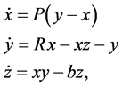(1)

where, , , and are positive constants, called the Prandtl, Rayleigh, and Biot numbers, respectively.

The Lorenz equations first arose in the study of the fluid flow of the atmosphere by Lorenz [1] . The system has been studied extensively. Virtually all texts discussing nonlinear differential equations and dynamical systems discuss the Lorenz equations in some manner. Robinson [2] , Glendinning [3] , and Jordan and Smith [4] are just a few. Although initially the system was used to model the atmosphere, the equations have also been used in models of lasers [5] , thermosyphons [6] , motors [7] , electric circuits [8] , chemical reactions [9] and osmosis [10] .

In what follows, a physical interpretation of x, y, and z is important. We use Lorenz’s Lorenz derives system (1) in [1] from a simplified version of a partial differential equation formed by Saltzman [11] . For system (1), Lorenz states:

In these equations, x is proportional to the intensity of the convective motion, while y is proportional to the temperature difference between the ascending and descending currents, similar signs of x and y denoting that warm fluid is rising and cold fluid is descending. The variable z is proportional to the distortion of the vertical temperature profile from linearity, a positive value indicating that the strongest gradients occur near the boundaries.

The Prandtl number, P, is given by, where k is the coefficient of thermal diffusivity and is the kinematic viscosity. The Rayleigh number determines whether heat is transferring primarily by conduction or convection and is given by

where g is the acceleration of gravity, is the coefficient of volume expansion, H is the height of fluid, and is a temperature contrast (refer to Saltzman [11] and Lorenz [1] for detailed explanations of the derivation of system (1) and meaning of the various parameters and variables). The Rayleigh number is the critical number governing the behavior of the Lorenz equations. Once R reaches a critical value, stable solutions of the system become unstable.

2. Review of Equilibrium Points of the Lorenz System and Local Stability Analysis

Solving

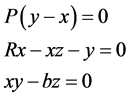(2)

yields the rest points (equilibrium points)

The Jacobian of system (1) is

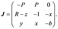(3)

Evaluated at, the Jacobian 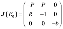has eigenvalues and

For to be unstable, we must have that

In the case that, it is straightforward to show that is globally asymptotically stable [3] .

We now assume that. Observe that with this assumption, the rest points will always exist.

Evaluated at and, respectively, the Jacobian is

(4)

The characteristic polynomials for both and are the same:

(5)

The calculations begin to illustrate the complexities of this system. The Lorenz system is often used to illustrate how a very “simple” system can lead to chaotic behavior. Equation (5) shows a dramatic difference between global and local behavior. With simple examples we can show that the stability of is truly local (rather than global) and provide numerical evidence that the system does not have any limit cycles.

Because the coefficients of (5) are all nonnegative, the solutions of (5) will all have negative real part by the Routh-Hurwitz theorem if

(6)

For our calculations, we will follow a typical convention and set and. Then, (6) becomes. Under these conditions are locally stable. Thus, to induce chaotic behavior in the Lorenz system, it is common to choose so that are unstable.

2.1. Example: Stable ()

Before addressing the unstable situation and incorporating a controller to eliminate chaos in system (1) when, we begin with an example with an R value so that are locally stable. For the example, we choose. For this value of R, we have the rest points and. The eigenvalues of the Jacobian of (1) evaluated at are −20.3408, 9.34082, and −2.266667. Because of the positive eigenvalue, is unstable. At the eigenvalues of the Jacobian are −13.3571, and so are locally stable.

In Figure 1, we illustrate the basins of attraction for. For the given value of, if is in the gray region, the solution satisfying the initial conditions converges to. On the other hand, if is in the black region, the solution satisfying the initial conditions converges to. Comment: All graphics and computations in this paper were done using Mathematica 10.0 [12] . If you would like a copy of the code, send a request to Jim Braselton at jbraselton@georgiasouthern.edu.

Note the “speckled” regions in Figure 1, in these regions we see that system (1) is highly sensitive to initial conditions. For some initial conditions, the solutions converge to but a slight change in the conditions can cause the solution to converge to and vice-versa.

The complexity of how the initial conditions affect the convergence of the solution to or is further illustrated in Figures 2-4. Because the z-coordinate of and are equal, the plot of z as a function of t in Figure 4 is the same regardless of whether the solution converges to or.

2.2. Example: Stable () Coexist with a Strange Attractor

Interestingly, it is possible for to be locally stable and yet the Lorenz equations will have a strange attractor.

For the and values typically used when studying the Lorenz system, for, are stable and coexist with a single strange attractor [13] . To illustrate the interesting situation, we set. For this value of R, we have the rest points and. The eigenvalues of the Jacobian of (1) evaluated at are −21.7558, 10.7558, and −2.266667. Because of the positive eigenvalue, is unstable. At the eigenvalues of the Jacobian are −13.6462, and so are locally stable.

In Figure 5 we illustrate the basins of attraction for. For the given value of, if

is in the gray region, the solution satisfying the initial conditions converges to. On the other hand, if is in the black region, the solution satisfying the initial conditions converges to. However, in the speckled region, the solution satisfying the initial conditions converges to the strange attractor which is illustrated in Figure 6.

3. A Quotient Controller

The chaos/strange attractors observed in the Lorenz system in the context of a model of the atmosphere are interpreted to mean that over long (and, frequently, short) periods of time, the weather is not predictable. Hence, controlling the solutions to the Lorenz system to eliminate chaos/strange attractors are interpreted there is a means by which to make weather forecasts more accurate over longer (and shorter) periods of time. Shen [14] , generalizes the Lorenz equations with two additional modes and analyzes a 5-dimensional Lorenz system. Shen’s 5-dimensional system exhibits strange attractors for larger R values than the original 3-dimensional Lorenz system. In other words, for some R values for which system (1) exhibits chaos, the corresponding 5-dimensional system analyzed by Shen does not. As with Shen, our goal is to eliminate chaos by reducing the value of R via a quotient controller as a perturbation of R. We do this by incorporating a quotient controller into y-equation of system (1).

We now incorporate a quotient controller of the form

(7)

into the y-equation in the Lorenz system. We use a quotient controller in the y-equation to control R rather than a linear control in the x-equations as done by Braselton and Wu [15] , because the y and z states are (theoretically) easily measurable (compared to x), while R is proportional to the external heat applied to the system. Therefore, the controller serves as an actuator to perturb the heat source. The quotient controller is applied to perturb the Rayleigh number, R, which is the key parameter to initiating chaos in the Lorenz system, as follows

(8)

where, , and are the Prandtl, Rayleigh, and Biot numbers, respectively, and is the feedback gain.

3.1. Local Stability Analysis

Solving

(9)

results in the equilibrium points

(10)

The Jacobian for (8) is

(11)

after dividing by, the characteristic polynomial of (11) evaluated at the equilibrium points (10) has the form, where

(12)

If, , , and are all positive and

(13)

then by the Routh-Hurwitz theorem, the real part of the roots of the characteristic polynomial of (11) evaluated at the equilibrium points (10) will all have negative real part and, consequently, will be locally stable.

The roots of have negative real part under the following conditions.

・ and

- and or

-

or

・ .

If these conditions are not satisfied, then the real part of the roots of the characteristic polynomial of (11) evaluated at the equilibrium points (10) will have a positive real part and, consequently, will be unstable. If initial conditions, , cause system (8) to converge to one of, then

because of the term in system (8), must be greater than 0 to avoid discontinuities in the solution to

the system.

The values and are frequently used when studying the Lorenz equations. Using these values we can rewrite the conditions above as

. (14)

Figure 7 shows a portion of the region where or For points in

the shaded region, the equilibrium points (10) will be locally stable. Also, if k is sufficiently large, will be locally stable, which is not illustrated in Figure 7. However, from a physical interpretation, smaller k values are preferred as they require less energy than larger k values. Large k-values can be interpreted as a “heavy-handed controller:” if enough power is applied to the system to cause it to stop, it will.

3.2. Example:

Using, , and, with, we find the rest points and . Evaluated at, the eigenvalues of the Jacobian of (8) when are and so that are unstable. Evaluated at, the Jacobian has eigenvalues, , and so is unstable as well (see Figure 8).

To stabilize the system, we first solve, which shows us that if,

will be locally stable (see Figure 9). We set. In this case,. Note that the addition of the controller changes the location of the rest points. The eigenvalues of the Jacobian of

(15)

evaluated at are, and so are locally stable (although their location has moved slightly from when their was no controller).

Numerically, we see that there is a ball centered at each of for which all trajectories starting in the ball converge to. However, the basin of attraction for each point is quite complex. Figure 10 shows the plot of for various values of. First, we solve system (8) using the initial conditions, and. We then plot in gray if the solution converges to and in black if the solution converges to.

The complexity of the basins of attractions are even more apparent when zooming in near one of the equilibria or zooming out as shown in Figure 11.

These figures provide numerical evidence that controlled system has no limit cycles. For those initial

conditions in the black region, the solutions converges to while for those solutions in the gray region, the solutions converge to. Of interest is the “speckled” regions. In these regions we see that system (8) is highly sensitive to initial conditions. For some initial conditions, the solutions converges to but a slight change in the conditions can cause the solution to converge to and vice-versa.

The initial conditions have a major affect on the convergence of a solution to or as is illustrated in Figures 12-14. Because the z-coordinate of and are equal, the plot of z as a function of t in Figure 14 is the same regardless of whether the solution converges to or.

To investigate the existence of a strange attractor as observed in Section 2.2, for each value in Figure 10, we drew a line from slightly before to slightly after. We then computed solutions satisfying, , and for 50 equally spaced points on each line and graphed them. In every case, the observed solution converged to or. For points in the “speckled” region, the solutions varied as to whether they converged to or. Thus, for this R value, we were not able to produce a strange attractor as we did in Section 2.2. Our conjecture is that periodic orbits do not exist and that all solutions converge to or.

3.3. Example: with Large k

Using, , and, with, we find the rest points and . Evaluated at, the eigenvalues of the Jacobian of (8) when are and so that are unstable. Evaluated at, the Jacobian has eigenvalues, , and so is unstable as well. From Figure 7, we see that we will be able to stabilize the system for k-values greater than approximately 0.35. In Section 3.4 that follows, we chose a small k-value to stabilize the system. In this case, choose a large k-value and choose. We choose this k-value because if a trajectory converges to or,

and for R-values in this range (), it is possible for to be stable and yet the system may have a strange attractor as we saw in Section 2.2. Thus, we expected that this controlled system may have a strange attractor as we saw with the corresponding non-controlled system. For this k-value, we obtain. The eigenvalues of the Jacobian evaluated at are,

, and.

Figure 15 illustrates the basin of attraction for various values of. In this case, observe that with large k, the boundary between and is specific and there is not a “speckled” region that was observed for smaller k values.

To investigate the stability of and, we followed the exact same procedure as in Section 2. Once again, we were not able to find a strange attractor leading us to believe that the stability of the limit set is global. The numerical evidence suggest that with a controller of this type, solutions will converge to either or. Even though converges to a number in the range where the uncontrolled system can have two stable equilibria and a strange attractor, for the controlled system we were surprised to see that the controlled system did not produce a strange attractor.

3.4. Example: with Small k

To investigate how implementing our controller affects the stability of solutions of the Lorenz equation, we have examined an extreme range of R and k-values hoping that these simulations indicate the the global behavior that we have numerically observed.

Our last example involves a large R-value and a small k-value. We repeat the example in Section 3.4 except we use. For this k-value, we obtain. The eigenvalues of the Jacobian evaluated at are and.

The situation appears to be similar to the situation discussed previously with small k-values. In Figure 16, observe the “speckled” region as before where solutions may converge to or with slight differences in the initial conditions.

As we did with the previous examples, to investigate the existence of a strange attractor as observed in Section 2.2, for each value in Figure 16, we drew a line from slightly before to slightly after. We then computed solutions satisfying, , and for 50 equally spaced points on each line and graphed them. In every case, the observed solution converged to or. For points in the “speckled” region, the solutions varied as to whether they converged to or. Thus, for this R value, we were not able to produce a strange attractor as we did in Section 2.2. We suspect that the stability is global in that all

solutions converge to or.

Note that we were able to produce “almost strange attractors” in the sense that the trajectories appeared to be chaotic at first-but eventually converged to either or in all our simulations.

4. Conclusions

In this paper, we revisited the three-dimensional Lorenz system. We illustrated how the Lorenz system can exhibit chaos (or, strange attractors) even when the non-trivial equilibrium points are locally stable.

We then introduced a closed loop quotient controller into the three-dimensional Lorenz system, computed the equilibrium points and analyzed their local stability. We use several examples to illustrate how cross-sections of the basins of attraction look for various parameter values. We then provided numerical evidence that with the

controller, the controlled Lorenz system cannot exhibit chaos if the equilibrium points are locally stable.

Our controller controlled the heat source, R. Of course, in the context of Earth’s atmosphere, the design and construction of a controller that could truly control Earth’s R-value would be an engineering miracle.

About the Computations

All computations were carried out using Mathematica Version 10 [12] . Readers can obtain the Mathematica notebooks used for the computations and graphics here by sending an email request to jbraselton@georgiasouthern.edu.

Acknowledgements

We thank the Editor and the referees for their comments.

Cite this paper

James Braselton,Yan Wu, (2016) Stabilizing the Lorenz Flows Using a Closed Loop Quotient Controller. Open Journal of Applied Sciences,06,560-578. doi: 10.4236/ojapps.2016.68056

References

- 1. Lorenz, E.N. (1963) Deterministic Non-Periodic Flows. Journal of the Atmospheric Sciences, 20, 130-141. http://dx.doi.org/10.1175/1520-0469(1963)020<0130:DNF>2.0.CO;2
- 2. Robinson, C. (1999) Dynamical Systems: Stability, Symbolic Dynamics, and Chaos. 2nd Edition, CRC Press LLC, Boca Raton, Florida.
- 3. Glendinning, P. (1994) Stability, Instability, and Chaos: An Introduction to the Theory of Nonlinear Differential Equations. Cambridge University Press, Cambridge. http://dx.doi.org/10.1017/CBO9780511626296
- 4. Jordan, D.W. and Smith, P. (2007) Nonlinear Ordinary Differential Equations: An Introduction for Scientists and Engineers. 4th Edition, Oxford University Press, New York.
- 5. Haken, H. (1975) Analogy between Higher Instabilities in Fluids and Lasers. Physics Letters A, 53, 77-78. http://dx.doi.org/10.1016/0375-9601(75)90353-9
- 6. Tanner, J.S. (2007) State Feedback Control of a Single-Loop Thermosyphon System via a Quotient Controller. Master’s Thesis, Georgia Southern University.
- 7. Hermati, N. (1994) Strange Attractors in Brushless DC Motors. IEEE Transactions on Circuits and Systems I: Fundamental Theory and Applications, 41, 40-45. http://dx.doi.org/10.1109/81.260218
- 8. Cuomo, K.M. and Oppenheim, A.V. (1993) Circuit Implementation of Synchronized Chaos with Applications to Communications. Physical Review Letters, 71, 65-68. http://dx.doi.org/10.1103/PhysRevLett.71.65
- 9. Poland, D. (1993) Cooperative Catalysis and Chemical Chaos: A Chemical Model for the Lorenz Equations. Physica D, 65, 86-99. http://dx.doi.org/10.1016/0167-2789(93)90006-M
- 10. Tzenov, S. (1994) Strange Attractors Characterizing the Osmotic Instability. arXiv:1406.0979.
- 11. Saltzman, B. (1962) Finite Amplitude Free Convection as an Initial Value Problem-I. Journal of the Atmospheric Sciences, 19, 329-342. http://dx.doi.org/10.1175/1520-0469(1962)019<0329:FAFCAA>2.0.CO;2
- 12. Wolfram Research (2016) Mathematica 10.0. Champaign, Illinois.
- 13. Sprott, J.C. (2013) Tri-Stability in the Lorenz System. Technical Report, Department of Physics, University of Wisconsin, Madison, Wisconsin. http://sprott.physics.wisc.edu/technote/tristab.htm
- 14. Shen, B.-W. (2014) Nonlinear Feedback in a Five-Dimensional Lorenz Model. Journal of the Atmospheric Sciences, 71, 1701-1723. http://dx.doi.org/10.1175/JAS-D-13-0223.1
- 15. Braselton, J. and Wu, Y. (2016) Applying Linear Controls to Chaotic Continuous Dynamical Systems. Open Journal of Applied Sciences, 6, 141-152. http://dx.doi.org/10.4236/ojapps.2016.63015