ABSTRACT

This paper research is the first part of the scientific theory that seeks to unify the sciences of physics with the minimal number of mathematical formulas as possible. We will prove that all equations of forces in nature can be concised in two mathematical formulas, no difference between gravitational or electrical forces or any other type of Types of conventional forces, and through the equivalence of the concepts of matrix and vector, in this theory we will be linking the four-dimensional forces equations with the classical physics as an introduction to connect the rest of the physical sciences.

Keywords:

Equations of Force, Gravity, Electromagnetism, Khromatic Theory, Maxwell’s Equations, Relativity

1. Introduction

Numerous of recent books in physics discourse the summarizing of Maxwell’s four equations into two equations, without addressing the possibility to generalize this concept to the rest of the forces, and work to link them with classical physics, which is the goal of publishing this research.

Whereas we cannot link all the physical sciences in one theory, unless the base upon which this theory was built represents a good and common ground for all of these sciences, So at the beginning will get to know some mathematical concepts (for example the relationship between the matrix and the vector) in a new and concise manner, with the remarks that we will deliberately ignore some proofs and details of those concepts to shorten the pages of this research that will exceed tens of pages.

In this part of the theory we will prove that all equations of force in nature belong basically to two basic mathematical formulas, on the Figure and, including Lagrange equation, which will we address in the coming research, and the results obtained in this research will be applied only to the electrical and magnetic forces, with no other ones, since these forces are the most prominent in the books of physics.

In the next parts we will explore the possibility of combining the theories of General Relativity and Quantum Mechanics with this theory in the minimal mathematical relationships as possible.

However, the purpose of publishing this paper can be summarized as follows

1) Introducing new mathematical ideas and concepts which will help to unify physics;

2) Unification of the physical sciences with as few equations as possible (in this part, most of the forces known as only two forms);

3) Linking modern physical science with ancient physics without resorting to any hypotheses (such as the stability of the speed of light in the theory of relativity).

2. Basic Notions

2.1. A.E Filed

In this paper, the space is called A.E space in n-dimensional with m-index filed, in this case. We suppose that the m-index filed vector in is defined by

where

is a complex orthogonal unit, that is defined by setting

are unit vectors in the directions.

In general, the space of two vectors and is defined as in n-dimensional with m, ρ mix-filed.

2.2. Theory

“The cross product of a set of vectors in any specified space equal to the Determinant of these vectors”

It mean that if

with And,

, then

2.3. Determinants and Dual Determinants

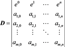
2.3.1. The Main Determinant

The main determinant of (m + 1) × (n) matrix has been defined. Denote by the sub determinant of the (m) × (m) matrix obtained from D by deleting the first row and choosing the -columns. Then, the main determinant of matrix denote as

where

m: the number of the vectors in the group;

―the numbers of columns which has been chosen.

2.3.2. The Dual Determinant of Matrix Denote as

and the dual sub determinant define by equation,

(2.1)

where

―the numbers of columns which has not been chosen.

or denotes the cyclic permutation symmetry.

Let,:, and, Then

Thus,

where,

► For example:

let,:

Then, from above equation we get

The magnitude or length of the vector in is defined as

From dot product, we get

:. Thus

The last equation equals the length of the vector in

2.3.3. Calculate the Dual to

From (2.1), we can define the dual vector by equation

3. Vector Properties in

3.1. Conversion to Matrix Form Property

3.1.1. Let Be Any Vector in, It Can Be Written as the Main Matrix in the Form

, where

3.1.2. The Dual Vector, It Can Be Written as the Dual Matrix in the Form

, then

3.2. The Mix Product Property

3.2.1. The Mix Cross-Product of Two Vectors and Is Defined by Setting

(3.1)

3.2.2. The Mix Dot-Product of Two Vectors and Is Defined by Setting

(3.2)

where,

From (2.1), we therefore get

(3.3)

► Now in the example at hand, we have

Let,

Then, the cross-product of two vectors and is defined as

(I)

On the other hand, we have from vector relations the equation

Here the last vector equals the Equation (1).

The dot-product of and is defined as

(II)

From (3.2), we therefore get

Here the new vector appearing on the right-hand side equals the Equation (II).

4. The Force Equations on A.E Filed

On A.E filed, there are only two types of forces namely cross and dot forces

4.1. Calculate the Cross Force F_cross

Let be 4-force in the form

Therefore

as

Then

(4.1)

According to the three-orthogonal vectors e¹, e², e³ we can rewrite the field vectors as

(4.2)

Now consider the equations

(4.3)

Thus, the Equation (4.1) becomes

we therefore get

(4.4)

4.2. Calculate the Dot Force F_dot

Let be 4-Force in the form

From Equation (3.2) we have

where

Using the three-orthogonal vectors e¹, e², e³ we can rewrite the transformation in Equation (4.2) and Equation (4.3) as

then we obtain

Thus

For the orthogonal unit vectors e¹, e², e³ the last equation becomes

(4.5)

where

► Let in our example

:

Then

,

thus from Equation (4.4) and Equation (4.5) we get

The last two equations equals the Equation (I) and the Equation (II).

5. The Relationships between the Force Equations on A.E Filed and the Conventional Force

5.1. Calculate the Conventional Ordinary Force

The 4-momentum P of a particle of mass m₀ at position moving at

velocity can be written as

The 3-velocity v of the particle is defined by, then

where is called an angular velocity vector of the rotating system,

թ is the 4-momentum of the coordinate system itself, թ = (թ₀, թ)

Thus

Now, we can rewrite last equation as the following

(5.1)

where

(5.2)

5.2. Comparison to Cross Force

If the Equation (5.1) is equivalent to the cross force equations in (4.4), we shall have

(5.3)

6. Some Special Results

6.1. Covariant Conventional Force

From comparison above, we have, thus

(6.1)

6.2. The Value of the Component f^o

From Equation (5.3) then,

(6.2)

6.3. The Equation of 4-Angular Velocity

Return above we have in the three-dimensional space

So, in the four-dimensional space time we Consider the and components are given by bold line, normal line, where

For E M case, Let A is the vector potential and թ = qA [1] then we get

(6.3.1)

(6.3.2)

6.4. The Value of թ₀

The sub determinant of angular velocity is defined by

From Equation (5.3) and Equation (4.3) we then get

which is equivalent to Equation (5.2).

where ∅ is scalar potential energy, so we can write the 4-coordinate momentum թ as,

For 4-vector potential A, we get [2]

6.5. Calculate the Dual to F'

We suppose that the dual force is defined by Equation (4.5) as the following

(6.4)

where

7. Conclusion

In A.E space, all force equations [3] (e.g. Coriolis Force, Lorentz force, ordinary force, Maxwell’s Equations and others) are elegantly represented by two simple equations

8. Discussion

8.1. E M Field Tenors

Using the transformation in Equation (4.2) and Equation (4.3), we obtain

The Equation (6.3.1) and Equation (6.3.2) follow that

By assuming that, then from Equation (5.3) we get

and so on. The overall result is [2]

By a similar argument, we can write the dual matrix as

8.2. Lorentz Force Law [4]

8.2.1. The First Force Equations on A.E Filed

Without the component, the Equation (5.1) becomes

to get the first E M Lorentz force law. Let

It follows that

8.2.2. The Second Force Equations on A.E Filed

Without the component, the the Equation (6.4) becomes

to get the second E M Lorentz force law. Let

It follows that

8.3. The 4-Field Equations in Tensor Notation [2]

According to the equations above, we can define 4-Maxwell’s Equations by suppose that

8.3.1. The Inhomogeneous E M Maxwell’s Equations

By vector triple product we have

But

, therefore

8.3.2. The Homogeneous Equations

From Equation (3.3) thus

, but

, then

Acknowledgements

I have named the new space in this paper as A.E (Abou Layla-Erdogan’s) as an expression of my thanks and appreciation for the Turkish President’s humanitarian attitudes towards my people and appreciation for my Turkish friends that supported me during my high study in Turkey.

Cite this paper

Abou Layla, A.K. (2018) Old Mechanics, Gravity, Electromagnetics and Relativity in One Theory: Part I. Journal of High Energy Physics, Gravitation and Cosmology, 4, 529-540. https://doi.org/10.4236/jhepgc.2018.43031

References

- 1. Abou Layla, A.K. (2017) Calclation the Exact Value of Gravitational Constant. LAP LAMBERT Academic Publishing. https://www.amazon.com/dp/3330337257/ref=cm_sw_r_fa_dp_U_-DfZAb9WVV8QK
- 2. Blau, M. (2017) Lecture Notes on General Relativity. http://www.blau.itp.unibe.ch/newlecturesGR.pdf
- 3. Abou Layla, A.K. (2017) Symmetry in Equations of Motion between the Atomic and Astronomical Models. Journal of High Energy Physics, Gravitation and Cosmology, 3, 328-338. http://www.scirp.org/journal/PaperDownload.aspx?paperID=75700 https://doi.org/10.4236/jhepgc.2017.32028
- 4. Wikipedia. Lorentz force. https://en.wikipedia.org/wiki/Lorentz_force