American Journal of Industrial and Business Management
Vol.06 No.05(2016), Article ID:66722,26 pages
10.4236/ajibm.2016.65058
Mediating Role of Route Characteristics on Effect of Low-Cost Carriers on the Airline Market in Kenya
Michael O. Aomo1, David O. Oima2, Moses N. Oginda3
1Directorate of Air Navigation Services, Kenya Civil Aviation Authority, Nairobi, Kenya
2Department of Accounting and Finance, Maseno University, Maseno, Kenya
3Department of Management Sciences, Maseno University, Maseno, Kenya

Copyright © 2016 by authors and Scientific Research Publishing Inc.
This work is licensed under the Creative Commons Attribution International License (CC BY).
http://creativecommons.org/licenses/by/4.0/


Received 29 April 2016; accepted 22 May 2016; published 25 May 2016
ABSTRACT
Studies show that low-cost carriers have gained 15.2% market shares while enplanement had increased by 38% following their emergence. Whereas frequency is directly influenced by airlines’ key factor such as turn-time, it, on the other hand, influences directly other airline market parameters. This proposes a mediation possibility. However, the mediating role of frequency on the relationship between turn-time on carriers’ market share, and the effect of low-cost carrier in Kenya was still unknown. The purpose of this study, therefore, was to investigate the mediating role of route characteristics on the effect of low-cost carriers on the airline market in Kenya. The specific objective of the study was to determine the effect of the mediating frequency on the relationship between turn-time and carriers’ market share. Using panel data of 2 airlines to capture both time-series and cross-sectional elements over the 72 months period, this paper will illustrate that frequency partially and off-the-scale significantly mediates turn-time-carrier’s market share relation. Path regression analysis is used to track the influence of the mediating route characteristics.
Keywords:
Carriers’ Market Share, Frequency, Low-Cost Carriers, Turn-Time

1. Introduction
While there had been a substantial body of research investigating this phenomenon in the US, Canada, Australia, and Europe, there had been little investigation of whether this phenomenon exists in other markets. Reference [1] recommended that there was a need to identify whether there is a low cost carrier effect in other markets. This paper therefore sought to investigate the mediating role of route characteristics on effect of low-cost carriers on the Kenyan airline market. According to [2] - [4] , low-cost carrier (LCC) is a discount airline that operates a point-to-point network, pays employees below the industry average wage, and offers no frills service. The low- cost airline model has proven that it is possible to follow different but disciplined business models and to deliver both service and financial results to world-class standards. Empirically, findings of many researchers have shown that the emergence of low cost carriers has had a profound impact in the aviation industry as seen in the works of [4] - [9] [11] [12] . For instance, it has resulted in increased enplanement by 38% and have gained 15.2% market share as reported by [4] and [5] respectively. On the other hand, in the markets such as Canada, North Atlantic routes and Netherlands, the low cost carriers have been found not to have any impact, e.g. [1] [13] [14] . The significance of turn-around punctuality is not only to reduce delays, but to maintain the linkage and stability of aircraft rotations [15] [16] . Whereas turn-time models provide useful information for schedule planning, fleet planning, operations planning, and economic and financial analysis, studies have concentrated on finding the effect of the emergence of low-cost carriers. None has actually investigated the impact that the low-cost carriers’ constructs, specifically turn-time, would have on their market share, and to a large extent, the mechanism through which it would achieve that. Several studies i.e. [17] - [21] have investigated about the models for the turn-around operations that would minimize delays, and consequently, costs. References [4] [6] [8] [12] employ descriptive statistics in analyzing their data on the effect of low cost carriers on the network carriers’ market share. On the other hand, studies by [9] [10] [22] have investigated on the frequency factor differently. Reference [9] considers it as independent variable on fare while [22] investigates it as an independent variable on airline market expansion, and finds a negative correlation between market concentration and flight frequency. Reference [10] treats it as a moderating variable on fare. Since theories posit frequency to be emanating from airlines’ turn-time while it also independently influences other aviation market parameters. This suggests that frequency would explain why a relationship between turn-time and any other variable occurs. However, the above cited studies had investigated frequency as either independent or moderating variable with respect to other airline market parameters. No study had considered it as a mediating variable in the relationships between turn- time and carriers’ market share. The specific objective of the study is, therefore, to examine the influence of the mediating frequency on the relationship between turn-time and carriers’ market share in the airline market.
The paper is arranged as follows: Section 2 briefly outlines the concept of low-cost carrier’s business model and the associated constructs, i.e. turn-time, frequency and market share. Previous studies are compared, contrasted, critiqued and the gap established. Section 3 outlines the methodology. Statistical tests for the assumptions of linear regressions, panel unit root tests, panel cointegration tests are performed. The mediating role of route characteristics is tracked, step by step, by use of path regression analyses in Section 4. The study is summarized, concluded and recommendations are made in Section 5.
2. Literature Review
This section reviews the concepts of low-cost carrier’s business model with an extension to specific constructs such as turn-time, frequency and the carrier’s market share. Previous empirical studies are highlighted. Comparisons, contrasting, critiquing and acknowledgement of the gap from the reviewed literature is established.
2.1. Low-Cost Carrier Business Model
According to [23] , the chief difference between low-cost carriers and traditional airlines, or full service carriers (FSCs), fall into three groups: service savings, operational savings and overhead savings. The low-cost model is characterized by specific product and operating features. Product features include: low, simple, and unrestricted fares; high frequencies; point-to-point flights; no interlining; ticketless travel utilizing travel agents and call centers; single-class, high density seating; no seat assignments; and no meals or free alcoholic drinks. Operating features include: single type aircraft with high utilization, secondary or uncongested airports served with short aircraft turns, short sector length, and competitive wages with profit sharing and high productivity [2] [4] [11] [24] [25] .
2.1.1. Turn-Time
Reference [15] defines turn-time as the period between the time an aircraft parks at the gate till it can pull out again with a new load of passengers and/or cargo. There are a number of key tasks to be carried out during this period: unloading and loading of passengers and luggage, safety and security checks, catering, cleaning and a variety of administrative tasks. The significance of turn-around punctuality is not only to reduce delays, but to maintain the linkage and stability of aircraft rotations [16] . Turn-time models provide useful information for schedule planning, fleet planning, operations planning, and economic and financial analysis. Reducing airplane turn-times means more efficient airplane utilization, particularly for airlines that emphasize point-to-point routes. Improved airplane utilization helps spread fixed ownership costs over an increased number of trips, reducing costs per seat-mile or per trip. More flights mean more paying passengers and, ultimately, more revenue. Benefits of shorter turn-times are significant for shorter average trip distances. In order to optimize airplane utilization, point-to-point carriers operate with significantly faster turn-times at the gate. A typical hub-and-spoke system requires longer turn-times to allow for synchronization between the feeder network and trunk routes [16] - [18] [21] [26] .
2.1.2. Frequency
Frequency is a central attribute when customers are determining mode choice [9] [26] [27] . Higher frequency of flights raises the value of the product to the passenger and increased value leads to higher demand and finally higher prices [10] . Passengers travelling on business have a high opportunity cost for travel and value the convenience increased frequency provides them. Hence, increased value leads to higher demand and finally higher prices [28] . It also facilitates a reduction in cost per transported unit due to the high fixed costs; higher frequency allows airlines to operate aircraft more efficiently and for longer utilization periods. Increased efficiency lowers an airline’s marginal cost and, thus, ticket prices [10] [29] . However, vessel capacity utilization is significantly lower for high-frequency routes [27] . A market that has a high concentration of passengers with high time costs (business travelers) might be served by smaller aircraft with greater frequency, while a market with a high concentration of low time cost passengers (leisure travelers) might be serviced by larger aircraft with lower frequency. As distance between the two end points increases, aircraft size increases and frequency decreases [30] . High rates of fleet utilization are a major factor in low-cost carriers’ business model. With high utilization, a low-cost airline will reduce costs significantly. The key for high utilization is to shorten the time between one flight and the other [31] since turn-times influence the number of trips an airplane can make in a given period of time [15] .
2.1.3. Carrier’s Market Share
References [32] and [33] pointed out that the reason for measuring the market share is to eliminate the impact of environmental factors which exert the same influence on all competing brands and thus allow a proper comparison of the competitive power of each. Calculating market shares assumes that the firm has clearly defined its reference market, i.e. the set of products or brands that compete with it. Reference [34] stated that incumbents (full service carriers) always attempt to retain the market share on the specific route low cost carrier airline joins by depressing their price. An increase in market share may allow airlines to exercise greater market power. With greater market power an airline can raise prices to increase its profits [35] .
2.2. Empirical Studies
References [4] [6] [8] [12] employed descriptive statistics in analyzing their data on the effect of low cost carriers on the network carriers’ market share. Reference [4] indicated that in the US, the low-cost carriers had claimed 15.2% market share from the incumbents’ market share within 5 years from 1998-2003. According to [8] , Spirit airlines claimed a market share of 4% within 3 months from American airlines following her entry into the market while [6] ’s findings show that the market share of low cost carriers has increased world-wide by about 22% over 33 years between early 1980s to 2013. Reference [12] reported that LCCs had accumulated around 34 per cent of the UK within 5 years from 1999-2004. According to [20] , scheduling every operations in the turn-around enhances a better performance and efficiency, while [17] remark that sensor technology or checkpoints, would enhance a better turnaround within highly automated environment. Reference [21] concluded that the minimum time of turnaround operations are in domestic-domestic flight type when passenger stair are used for disembarking and air-bridge for boarding. Reference [18] supported cooperation between a variety of tactical decision makers since it would deliver an efficient ground handling multi-fleet management structure. According to [19] , the automatic assignment strategy would give a better result in terms of minimum departure delays. On the other hand, reference [10] considered frequency as independent variable on fare while [9] treated it as a moderating variable on fare. Reference [22] investigated frequency as an independent variable on airline market expansion. Reference [22] found a negative relationship between market concentration and flight frequency. Reference [10] found out that the frequency variable is highly significant and has a negative impact on airfare per kilometer, and is inelastic in relation to price. According to [9] , the effect of the frequency of flights on a route, served by a particular carrier, is positive and significant at the 1 percent level over each fare percentile.
Since theories posit frequency to be emanating from airlines’ turn-time, and that frequency directly influences the airline market parameters, it therefore suggests that frequency would explain why a relationship between turn-time and any other variable occurs. However, the studies have investigated frequency as either independent or moderating variable with respect to other airline market parameters. No study had considered it as a mediating variable in the relationships between turn-time and carriers’ market share.
3. Research Methodology
This section addresses the research design, target population, type of data, statistical tests, and model specification.
3.1. Research Design, Target Population and Type of Data
The study adapted longitudinal design. Reference [36] defines longitudinal design as a time series correlational research design. Longitudinal research design describes patterns of change and helps establish the direction and magnitude of causal relationships [36] - [38] . Measurements are taken on each variable over two or more distinct time periods. This allows the researcher to measure change in variables over time. The target population of this study was 2 airlines i.e. Fly540, that formally operates as a low-cost carrier and Jetlink Aviation, which met the ICAO definition of a low-cost carrier in terms of operations but never used the term in marketing itself. Their data over a period of 72 months for the year 2007-2012 were used in the analysis. Sources of data were airlines statistics as maintained by the Kenya Civil Aviation Authority (KCAA).
3.2. Statistical Tests
Testing the Assumptions of Linear Regression
There are four principal assumptions which justify the use of linear regression models for purposes of inference or prediction. If any of these assumptions is violated, then the forecasts, confidence intervals, and scientific insights yielded by a regression model may be (at best) inefficient or (at worst) seriously biased or misleading [39] [40] . These assumptions are: (1) normality of the error distribution, (2) linearity and additivity of the relationship between dependent and independent variables, (3) statistical independence of the errors, and (4) homoscedasticity (constant variance) of the errors.
1) Test for Normality of the error distribution
Violations of normality create problems for determining whether model coefficients are significantly different from zero and for calculating confidence intervals for forecasts. Since parameter estimation is based on the minimization of squared error, a few extreme observations can exert a disproportionate influence on parameter estimates [40] [41] . Calculation of confidence intervals and various significance tests for coefficients are all based on the assumptions of normally distributed errors [42] [43] . If the error distribution is significantly non-normal, confidence intervals may be too wide or too narrow. In this study, the researcher used Jarque-Bera statistical tests for normality. Jarque-Bera test statistic measures the difference of the skewness and kurtosis of the series with those from the normal distribution [44] ; the Jarque-Bera statistic should not be significant in cases of normal distribution. The statistic is computed as:
 (1)
(1)
where S is the skewness, and K is the kurtosis.
However, real data, especially time series data, rarely has errors that are perfectly normally distributed, and it may not be possible to fit your data with a model whose errors do not violate the normality assumption at the 0.05 level of significance [40] [45] . This was observed even after transforming the data into the natural logs as shown in Table 1 and Table 2, the transformed natural logs of the variables could still not reject the null hypothesis at 5% significance. The researcher then settled on the [39] ’s and [40] ’s conclusion that it is usually better to focus more on the violations of the other assumptions since normality is a very minor concern.
2) Tests for Linearity or Additivity
Violations of linearity or additivity are extremely serious. If one fits a linear model to data which are nonlinearly or non-additively related, your predictions are likely to be seriously in error. In order to test for linearity, the researcher adopted Ramsey RESET (Regression Specification Error Test) to detect any incorrect functional form as proposed by [46] . The RESET Stability tests statistics indicated no evidence of non-linearity as shown in Tables 3-5, each table representing a linear association as proposed from the path regression analyses shown in Figure 1(a) and Figure 1(b).
In all the three analyses, i.e. Tables 3-5, the t-statistics strongly rejected any evidence of non-linearity.
 (a)
(a)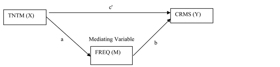 (b)
(b)
Figure 1. (a) Path Analysis Diagram for the direct effect of turn-time on carriers “market share”; (b) Path Analysis Diagram for the mediated effect of turn-time on carriers “market share”.

Table 1. First results of normality test using Jarque-Bera.
Table 2. Second results of normality test using Jarque-Bera.
Table 3. Ramsey RESET Linearity Test Results on the association between CRMS and TNTM.
Table 4. Ramsey RESET linearity test results on the association between FREQ and TNTM.
Table 5. Ramsey RESET linearity test results on the association between CRMS, TNTM and FREQ.
3) Statistical independence of the errors
When data are ordered―for example, when sequential observations represent Monday, Tuesday, and Wed- nesday―then the neighboring error terms may turn out to be correlated. This phenomenon is called serial correlation [44] [45] . If left untreated, serial correlation can do two bad things: reported standard errors and t-statistics can be quite far off, and under certain circumstances, the estimated regression coefficients can be quite badly biased. While using the Durbin-Watson statistical test for serial correlation, under the null hypothesis (no serial correlation) the Durbin-Watson centers around 2.0 rather than 0. If the serial correlation coefficient is zero, the Durbin-Watson is about 2. As the serial correlation coefficient heads toward 1.0, the Durbin-Watson heads toward 0.
4) Homoscedasticity (constant variance) of the errors
OLS makes the assumption that the variance of the error term is constant (Homoscedasticity). If the error terms do not have constant variance, they are said to be heteroscedastic. Heteroscedasticity does not cause ordinary least squares coefficient estimates to be biased, although it can cause ordinary least squares estimates of the variance (and, thus, standard errors) of the coefficients to be biased, possibly above or below the true or population variance [47] [48] . Thus, regression analysis using heteroscedastic data will still provide an unbiased estimate for the relationship between the predictor variable and the outcome, but standard errors and therefore inferences obtained from data analysis are suspect. Biased standard errors lead to biased inference, so results of hypothesis tests are possibly wrong. If OLS is performed on a heteroscedastic data set, yielding biased standard error estimation, a researcher might fail to reject a null hypothesis at a given significance level, when that null hypothesis was actually uncharacteristic of the actual population (making a type II error).
Heterokedasticity, serial correlations and presence of outliers were never perceived by the researcher to be problems at all due to the fact that Fully Modified Ordinary Least Squares (FMOLS) had been adopted in the panel cointegrating equations as outlined by [49] - [52] . This method modifies least squares to account for serial correlation effects and for the endogeneity in the regressors that results from the existence of a cointegrating relationship, as well robustic in dealing with the outliers.
5) Panel Unit Root Tests
While dealing with panel data, which is usually time series in nature, researcher may have to find out if the data is stationary [53] . Stationarity of data is when the mean, variance and covariance are time invariant (they do not change over time). This was done by use of panel unit root tests; Yt is regressed on its lagged value Yt?1 and then checked if the estimated slope coefficient is statistically equal to 1. If not, then Yt is nonstationary. This then requires first differencing of Yt which is then regressed on Yt?1, if the slope coefficient is 0, then Yt is nonstationary, and if it negative, then Yt is stationary [44] [45] . Any series that is not stationary is said to be nonstationary.
PP Fisher Panel unit root testing was performed on the three variables. The results showed that turn-time was stationary at order 0, while the other 2 (frequency, and carrier’s market share) were stationary at order 1. The following 5 tables (Tables 6-10) show the results of the panel unit root analysis for the series:
From Table 6, the results failed to reject null hypothesis of presence of a unit root in the series. Thus, first differencing was necessary as follows:
After first differencing, Table 7 indicates that the null hypothesis of the presence of a unit root was strongly rejected.
Table 8 indicates that the null hypothesis of the presence of a unit root was strongly rejected.
Table 9 indicates that the test failed to reject the null hypothesis of the presence of a unit root. Further differencing was then required as shown in the Table 10.
After first differencing, Table 10 indicates that the null hypothesis of the presence of a unit root was strongly rejected.
6) Panel Cointegration Tests
The finding that many macro time series may contain a unit root has spurred the development of the theory of non-stationary time series analysis [44] . Reference [54] pointed out that a linear combination of two or more
Table 6. Panel Unit Root Test Results for the zero-order CRMS series.
Source: Field data, 2016.
Table 7. Panel unit root test results for the first-order CRMS series.
Source: Researcher, 2016.
Table 8. Panel unit root test results for the zero-order TNTM series.
Source: Researcher, 2016.
Table 9. Panel unit root test results for the zero-order FREQ series.
Source: Researcher, 2016.
Table 10. Panel unit root test results for the first-order FREQ series.
Source: Researcher, 2016.
non-stationary series may be stationary. If such a stationary linear combination exists, the non-stationary time series are said to be cointegrated. The stationary linear combination is interpreted as a long-run equilibrium relationship among the variables. Given that most of variables were not stationary at order zero, it was necessary to carry out cointegration tests before deploying the more favorable panel cointegrating regression due to its more accuracy in estimations. The panel cointegration tests were carried out by use of Pedroni Residual Cointegration Tests that evaluate the null hypothesis of no cointegration at the conventional size of p < 0.05 against both the homogeneous and the heterogeneous alternatives (see Tables 11-13 for the results).
In this case, nine of the eleven statistics rejected the null hypothesis of no cointegration in Table 11.
The results in Table 12 show that five of the eleven statistics rejected the null hypothesis of no cointegration at the conventional size of 0.05.
The results in Table 13 indicate that nine of the eleven statistics rejected the null hypothesis of no cointegration at the conventional size of 0.05.
Table 11. Panel (pedroni residual) cointegration test results for the combined CRMS and TNTM series.
Table 12. Panel (pedroni residual) cointegration test results for the combined CRMS, TNTM and FREQ series.
Table 13. Panel (pedroni residual) cointegration test results for the combined FREQ and TNTM series.
3.3. Mediation Regression Model Specification
A mediation model offers an explanation for how, or why, two variables are related where an intervening or mediating variable, M, is hypothesized to be intermediate in the relation between an independent variable, X, and an outcome, Y [55] . More recent research has supported tests for statistical mediation based on coefficients from two or more of the following equations [56] [57] :
 (2)
(2)
 (3)
(3)
 (4)
(4)
where:
M is the mediating variable;
c is the overall (total) effect of the independent variable X on Y;
c' is the (direct) effect of the independent variable X on Y controlling for M;
b is the effect of the mediating variable on Y;
a is the effect of the independent variable X on the mediator;
β is the intercept for each equation; and
ε is corresponding residuals in each equation.
Thus, the following path analysis diagrams were used to develop the three regression equations to track the influence of the mediator variable, frequency, on the relationship between the turn-time and carriers’ market share:
Consequently, the following 3 regression equations will be:
To test if TNTM predicts CRMS → (5)
(5)
To test if TNTM predicts FREQ → (6)
(6)
To test if TNTM still predicts CRMS, when Mediator
(FREQ) is in the model → (7)
(7)
In the first regression, the significance of the path X to the dependent variable Y is examined. In the second regression, the significance of the path from X to M is examined. Finally, the significance of the path M to Y is examined in the third regression by using X and M as predictors of Y by use of simultaneous entry method. Simultaneous entry allows for controlling the effect of X while the effect of M on Y is examined, and controlling the effect of M while the effect of X on Y is examined. The results are then compared, that is, the relative effect of X on Y (when M is controlled in the third equation) to the effect of X on Y (when M is not controlled in the first equation). If the path X to Y in the third equation is reduced to zero, it provides strong evidence for a single, dominant mediator. If the residual path X to Y is not zero, it indicates that multiple mediating factors may be operating. The degree to which the effect is reduced (i.e. the change in the regression coefficient in Equation 3.4 versus the regression coefficient in Equation 3.2) indicates how powerful the mediator is [57] [58] .
Reference [59] cited that prior to using path analytic regression techniques, Pearson correlations among variables in the model are examined. The predictor variable must be significantly associated with the dependent variable (although this is not always a must condition as stated by [56] ) and with the mediator. Results in Table 14 indicate that turn-time is negatively correlated with both frequency and carrier market share, though the correlation is insignificant with respect to carrier’s market share, as shown by the value (r = −0.27, p-value of 0.001) and (r = −0.04, p-value = 0.596). This means that if turn-time is enhanced, both frequency and the carrier market share will reduce, but frequency will be more reduced. However, there is a strong significant positive correlation between frequency and carrier’s market share as shown by the value (r = 0.82, p-value = 0.000). This means that if frequency is enhanced, the carrier market share will be enhanced too.
Table 14. Correlational analysis between turn-time, frequency and Carrier’s market share.
3.4. Decision Criterion
M completely mediates X-Y relation if all the three conditions are met: (1) X predicts Y, (2) X predicts M, and (3), X no longer predicts Y, but M does when both X and M are used to predict Y [59] - [61] . M partially mediates X-Y relation if all the three conditions are met: (1) X predicts Y, (2) X predicts M, and (3), both X and M predict Y, but X have a smaller regression coefficient when both X and M are used to predict Y than when only X is used. M does not mediate X-Y relation if any of the three conditions are met: (1) X does not predict M, (2) M does not predict Y, and (3), the regression coefficient of X remain the same before and after M is used to predict Y.
Accordingly to [60] and [62] emphasized that since X predicts Z (mediating variable), there will be collinearity problem when they are both used in the same equation. In extreme cases, the researcher might not be able to fit the model. This problem can be sorted by increasing sample size and/or number of observations, or by use of panel data [48] [60] . Results in Table 15 showed VIF of 1.449. A commonly given rule of thumb is that VIFs of 10 or higher may be a reason for concern [63] . This is, however, just a rule of thumb; reference [64] says he gets concerned when the VIF is over 2.5. Since VIFs in this case is less than 1.5, the study concluded that there is no multicollinearity problem between the variables.
4. Results and Discussions
4.1. Descriptive Statistics
From Table 16, the mean of carriers’ market share is 13.25% which is about 5% lower than those low-cost carriers in Middle East, which is about 18.5% as reported by [3] , while turn-time has a mean of 32.60 minutes, this
Table 15. An examination of Collinearity between turn-time and frequency.
Table 16. Summary of the descriptive statistics.
is different from [3] ’s finding of 46.0 minutes averaged turn-around time for the US low-cost carriers. Frequency has a mean of 204.91 scheduled flights over the period. Median is the middle value (or average of the two middle values) of the series when the values are ordered from the smallest to the largest. The median of carrier’s market share is 12%, while turn-time has a median of 29 minutes. Frequency has a median of 229.5 number of scheduled flights over the period. Std. Dev. (standard deviation) is a measure of dispersion or spread in the series. The standard deviation is given by:
 (8)
(8)
where N is the number of observations in the current sample and  is the mean of the series. The standard deviation of carrier market share is 7.48 seats, while turn-time has a standard deviation of 11.89 minutes. Frequency has a standard deviation of 85.49 scheduled flights over the period. Skewness is a measure of asymmetry of the distribution of the series around its mean. Skewness is computed as:
 (9)
(9)
where σ is an estimator for the standard deviation that is based on the biased estimator, for the
Variance . The skewness of a symmetric distribution, such as the normal distribution, is
zero. Positive skewness means that the distribution has a long right tail and negative skewness implies that the distribution has a long left tail [42] [65] [66] . Carrier market share, turn-time are positively skewed as indicated by the values 0.74 and 0.39 respectively. This means that the mass of the distribution is concentrated on the right; carrier market share being the most positively skewed while load factor being the least positively skewed. On the other hand, frequency is negatively skewed as shown by the value −0.56, this implies that mass of the distribution is concentrated on the left. Kurtosis measures the peakedness or flatness of the distribution of the series. Kurtosis is computed as:
 (10)
(10)
where is σ again based on the biased estimator for the variance. The kurtosis of the normal distribution is 3 [44] . If the kurtosis exceeds 3, the distribution is peaked (leptokurtic) relative to the normal; if the kurtosis is less than 3, the distribution is flat (platykurtic) relative to the normal. All variables are platykurtic as indicated by 2.59 for carrier market share, 1.80 and 2.03 for turn-time and frequency respectively. This implies the variables have large standard deviations.
4.2. Inferential Analysis
It is well known that many economic time series are difference stationary which produce misleading results, with conventional Wald tests for coefficient significance spuriously showing a significant relationship between unrelated series [67] [68] . Reference [54] note that a linear combination of two or more I(1) series may be cointegrated, and such linear combination yields a long-run relationship between the variables. References [49] [50] [52] [68] suggested the use Fully Modified OLS (FMOLS) to provide optimal estimates of cointegrating regressions. The method modifies least squares to account for serial correlation effects and for the endogeneity in the regressors that results from the existence of a cointegrating relationship. Thus, in the following analyses, the researcher adopted FMOLS in the panel cointegrating regressions to overcome the problems of heterokedasticity, serial correlations and the outliers which are common with ordinary least squares (OLS). By combining time series of cross-section observations, panel data give more informative data, more variability, less collinearity among variables, more degrees of freedom and more efficiency [69] [70] . Panel data presents two big advantages over ordinary time series or cross section data. The obvious advantage is that panel data frequently has lots and lots of observations. The not always obvious advantage is that in certain circumstances panel data allows you to control for unobservable that would otherwise mess up your regression estimation. A key assumption in most applications of least squares regression is that there aren’t any omitted variables which are correlated with the included explanatory variables. (Omitted variables cause least squares estimates to be biased.) The usual problem is that if you don’t observe a variable, you don’t have much choice but to omit it from the regression. Panel data allows for the use of fixed effects to make up for the omitted variable.
Analysis of the effect of frequency as a mediator on the Relationship between Turn-time and Carrier Market Share
To examine the influence of the mediating frequency on the relationship between turn-time and carriers’ market share, the following 3 regression equations will be:
To test if TNTM predicts CRMS → (11)
(11)
To test if TNTM predicts FREQ→ (12)
(12)
To test if TNTM still predicts CRMS,
when Mediator (FREQ) is in the model → (13)
(13)
STEP 1: Finding out the effect of turn-time on carrier’s market share as denoted by the equation 
The results of the regression analysis in Table 17 indicate that turn-time is an off-the-scale significant negative predictor of carrier’s market share as indicated by β = −0.9382, t-statistic of −6.9368 against a p-value of 0.0000. This implies that any additional 1 minute of turn-time will result in the reduction of market share by −0.94%. The standard error which is a measure of uncertainty about the true value of the regression (turn-time) coefficient is 0.14%, while the standard error of the regression, which is the estimated standard deviation of the error term, for this equation is 5.98%. The R2 is 0.364 and the adjusted R2 is 0.355, the difference in this case being 0.009, and according to [72] , this model is valid and stable for prediction. Thus, the regression accounts for 36.4% of the carrier’s market share. This is supported by the fact that the standard deviation of the dependent variable is just slightly greater than the standard error of the regression (i.e. 7.47 is slightly greater than 5.99). Therefore, the model equation for this relationship is:
Table 17. Regression results of the effect of Turn-time on the carrier’s market share.
where: C represents the individual cross-section fixed effect, and is as follows:
and equation_01_efct is the S.E. of the regression and is equal to 5.98.
STEP 2: Finding out the effect of turn-time on frequency as denoted by the equation 
Results as shown in Table 18 indicate that turn-time is an off-the-scale significant negative predictor of frequency as shown by β = −9.94 with t-statistic of −5.8313 against a p-value of 0.000. This implies that any additional 1 minute in turn-time will result in a monthly frequency decrease of 9.94 scheduled flights. The standard error of the turn-time coefficient estimate is 1.70; while the standard error of the regression is 71.75 scheduled flights. The R2 is 0.2870 and the adjusted R2 is 0.2767. The shrinkage in this case is 0.0103, and therefore is fairly stable according to [72] . Thus, the regression accounts for 28.7% of the frequency. This is supported by the fact that the standard deviation of the dependent variable is slightly larger than the standard error of the regression (i.e. 84.36 is slightly greater than 71.75). The study therefore developed the following analytic model for predicting frequency:
 (15)
(15)
where: C represents the individual cross-section fixed effects, and is as follows:
and equation_02_efct is the S.E. of the regression and is equal to 71.75
STEP 3: Finding out the effect of the mediating frequency on the relationship between carrier’s market share and turn-time as denoted by the equation 
Table 19 indicates that turn-time is a negative predictor of carrier’s market share with β = −0.3079 as indicated by the t-statistic of −2.8402 against a p-value of 0.0052, while frequency is an off-the-scale significant positive predictor with β = 0.0606 as indicated by the t-statistic of 7.8528 against a p-value of 0.0000. This implies that any additional 1 minute in turn-time will result in a monthly carrier’s market share decrease of 0.31%. On the other hand, any additional 1 scheduled flight in the frequency will result in a monthly increase of carrier’s market share by 0.06%. The standard error of turn-time coefficient estimate is 0.11; while the standard error of frequency effect estimate is 0.01. The standard error of the regression fit is 3.74%. The R2 is 0.7530 and the adjusted R2 is 0.7476. The difference in this case being 0.0054 which shows good stability for prediction as suggested by [72] . Thus, the regression accounts for 75.30% of the carrier’s market share. This is supported by the fact that the standard deviation of the dependent variable is by far much larger than the standard error of the regression (i.e. 7.44 is far much larger than, twice the size of, 3.74). Thus, the analytic model for predicting carrier’s market share is:
 (16)
(16)
where: C represents the individual cross-section fixed effect, and are as follows:
and equation_03_efct is the S.E. of the regression and is equal to 3.74.
Table 18. Regression results of the effect of turn-time on frequency.
Table 19. Regression results of the effect of the mediating frequency on the relationship between carrier’s market share and turn-time.
Summary of the path regression analyses for the mediating variable
Thus, as shown in Figure 2, the summary of the path regression analyses for the mediating frequency will be as follows:
 (17)
(17)
 (18)
(18)
 (19)
(19)
4.2.1. Conclusion Based on Baron and Kenny (1986) Approach
Reference [57] considers the intermediate variable Z to be a mediator if: (1) H0(1): c = 0 is rejected (Y is associated with X); (2) H0(2): a = 0 is rejected (Z is associated with X); and (3) H0(3): b = 0 is rejected (Y is associated with the Z conditional on X). The satisfaction of these conditions indicates that there is a mediating effect of X on Y through Z. If all three of these steps are met and H0(4): c′ = 0 is rejected, then the data are consistent with the hypothesis that variable Z partially mediates the X-Y relationship, and if H0(4): c′ = 0 is not rejected, then complete mediation is indicated. Thus, from Baron and Kenny (1986) approach, the study concluded that frequency partially mediates the turn-time-carrier’s market share relationship since all the 4 null hypotheses were rejected.
4.2.2. Analysis of the Mediating Effect of Frequency on the Relationship between Turn-Time and Carrier’s Market Share Using the Judd and Kenny (1981) Indirect Effect
Reference [57] ’s approach is the general approach many researchers use. There are potential problems with this approach, however. One problem is that we do not ever really test the significance of the indirect pathway―that X affects Y through the compound pathway of a and b. A second problem is that the Barron and Kenny approach tends to miss some true mediation effects (Type II errors) [56] . An alternative, and preferable approach, is to calculate the indirect effect and test it for significance. The regression coefficient for the indirect effect represents the change in Y for every unit change in X that is mediated by M. Reference [71] suggested computing the difference between two regression coefficients. To do this, two regressions are required.
The approach involves subtracting the partial regression coefficient obtained in Model 1, c' from the simple regression coefficient obtained from Model 2, c. Note that both represent the effect of X on Y but that cis the zero-order coefficient from the simple regression and c' is the partial regression coefficient from a multiple regression. The indirect effect is the difference between these two coefficients (Refer to Table 20):
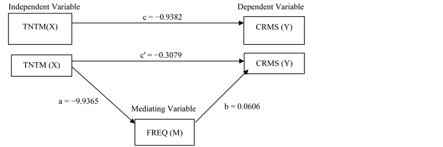
Figure 2. Estimated path analysis diagram for the mediated effect of turn-time on carriers’ market share.
Table 20. Regression equation depiction of the Judd and Kenny difference of coefficients approach.
Source: Researcher, 2016.
 (20)
(20)

As shown by Table 21, when only turn-time is included in the equation, its effect is −0.9382. However, when frequency is introduced, while controlling for turn-time, the coefficient of turn-time reduces to −0.3079. Thus, the introduction of an intervening variable, frequency, reduces the turn-time effect by −0.6303, i.e. (−0.9382 minus −0.3079). This means that out of all (100%) effects the turn-time will have on carrier’s market share, 67.18% of that effect is attributable to frequency as shown in Figure 3.
4.2.3. Analysis of the Mediating Effect of Frequency on the Relationship between Turn-Time and Carrier’s Market Share Using the Sobel (1982) Coefficient Approach
Sobel (1982) approach calculates the indirect effect by multiplying two regression coefficients. The two coefficients are obtained from two regression models stated in Table 22.
In the Sobel approach, Model 2 involves the relationship between X and M. A product is formed by multiplying two coefficients together, the partial regression effect for M predicting Y, b1, and the simple coefficient for X predicting M, a:
 (21)
(21)
As summarized in Table 23, the total effect of turn-time on frequency, a, is −9.9365; while the coefficient of frequency, while controlling for turn-time, is 0.0606. Thus, the product of a1b1 is −0.6018, and the proportion with respect to c is 0.6414. This means out of all (100%) effects (total effect), the turn-time will have on carrier’s market share, 64.14% of that effect is attributable to frequency.
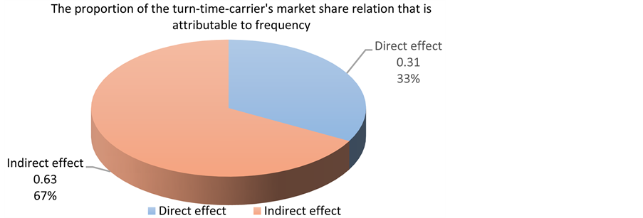
Figure 3. The proportion of turn-time-carrier’s market share relation that is attributable to frequency. Source: Researcher, 2016.
Table 21. Analysis of the portion attributable to frequency using Judd and Kenny (1981).
Source: Researcher, 2016.
Table 22. Regression equation depiction of the Sobel product of coefficients approach.
Source: Researcher, 2016.
Table 23. Analysis of the mediating impact of frequency using Sobel (1982) coefficient approach.
Source: Researcher, 2016.
4.2.4. Sobel Test for the Significance of Mediation
The Sobel test determines whether the mediator variable significantly carries the influence of an independent variable to a dependent variable; i.e., whether the indirect effect of the independent variable on the dependent variable through the mediator variable is significant [60] [73] . The following formula is used:
 (22)
(22)
where a and b are the standardized regression coefficients, and sa and sb are their standard errors. The researcher used Sobel test statistics Calculatorand results show the Sobel test statistic, and both one-tailed and two-tailed probability values as shown in Table 24.
From Table 24, the Sobel test statistics of −4.6821 against a one-tailed p-value of 0.0000 or a two-tailed p-value of 0.0000 implies that the null hypothesis of the indirect effect coefficient being zero is strongly rejected. Thus, the mediating effect of frequency is off-the-scale significant.
4.2.5. Conclusion on the Mediating Effect of Frequency on the Turn-Time-Carrier’s Market Share Relationship
M (frequency) partially, but off-the-scale significantly, mediates X (turn-time)?Y (carrier’s market share) relation by 64.14% since all the 4 conditions have been met: (1), X (turn-time) predicts Y (carrier’s market share); (2), X (turn-time) predicts M (frequency); (3), both X (turn-time) and M (frequency) predict Y, but X (turn-time) have a smaller regression coefficient when both X (turn-time) and M (frequency) are used to predict Y (carrier’s market share)than when only X (turn-time) is used; and (4), the indirect effect coefficient is off-the-scale significant. This finding is different from the findings of [9] [10] [22] since they have investigated on the frequency variable differently. Reference [10] considers it as independent variable on fare found out that the frequency variable is highly significant and has a negative impact on airfare per kilometer, and is inelastic in relation to price. Reference [9] treats it as a moderating variable on fare the effect of the frequency of flights on a route, served by a particular carrier, is positive and significant at the 1 percent level over each fare percentile. Reference [22] investigated it as an independent variable on aviation market expansion and found a negative relationship between market concentration and flight frequency. The current study results offer evidence indicating that frequency partially and off-the-scale significantly mediates turn-time-carrier’s market share relation by 64.14 per cent, in line with the researcher’s expectation that frequency is an important mechanism through which turn-time influence carrier’s market share
5. Summary, Conclusions and Recommendations
Correlational analyses indicate that: there is a very weak negative correlation between turn-time and carrier’s market share; turn-time is significantly negatively correlated with frequency; there is a very strong significant positive correlation between frequency and carrier market share. The current study, therefore, has established that: turn-time is a significant negative predictor of carrier’s market share while frequency partially and off-the- scale significantly mediates turn-time-carrier’s market share relation by 64.14 per cent. This is the first study reporting on the mediating role of route characteristics on the effect of low-cost carrier on the airline market in Kenya. Based on the conclusion, airlines, therefore, need to adopt very efficient turn-around models since for high airplane utilization to be realized, the time between one flight and another must be shortened. This requires good operating systems to ensure that all necessary ground handling procedures can be completed during a limited period. One way to simplify ground handling procedures and cut down the time gap is by using one type of aircraft for the airline’s whole fleet. Secondly, since frequency of service has an effect on competitors’ market share, airlines need to increase the number of scheduled flights during busy seasons like holidays and week-ends. The researcher recommends similar studies should be designed with a view to replicating the results of this research within the wider setting of the entire Kenyan aviation industry to include the full service carriers. Finally,
(a) (b)
Table 24. The Results of the Sobel Test for significance of the mediating frequency.
Source: Researcher, 2016.
whereas frequency partially and off-the-scale significantly mediates turn-time and carrier’s market relation share relation by 64%, the researcher suggests that there is need to investigate whether the remaining 36% is solely the direct effect of turn-time, or there are still some other mediating factors between the turn-time-carrier’s market share relation.
Cite this paper
Michael O. Aomo,David O. Oima,Moses N. Oginda, (2016) Mediating Role of Route Characteristics on Effect of Low-Cost Carriers on the Airline Market in Kenya. American Journal of Industrial and Business Management,06,614-639. doi: 10.4236/ajibm.2016.65058
References
- 1. Mentzer, M.S. (2013) The Elusive Low Cost Carrier Effect in the Trans-Atlantic Airline Market. Journal of Aviation Management and Education, 2, 11-19.
- 2. Rosenstein, D.E. (2013) The Changing Low-Cost Airline Model: An Analysis of Spirit Airlines. Aviation Technology Graduate Student Publications. Department of Aviation University, Purdue University: e-pubs.
http://docs.lib.purdue.edu/atgrads/19 - 3. Dresner, M. (2013) Low-Cost Carriers. University of Maryland, Tokyo.
- 4. O’Connell, J. and Williams, G. (2007) The Strategic Response of Full Service Airlines to the Low Cost Carrier Threat and the Perception of Passengers to Each Type of Carrier. PhD Thesis, School of Engineering, Cranfield University, Cranfield.
- 5. InterVistas Consulting Group (2014) Transforming Intra-African Air Connectivity: The Economic Benefits of Implementing the Yamoussoukro Decision. IATA, Geneva.
- 6. Israel, M. (2015) International Low-Cost Airline Market Research. Tarmac Aviation, Germany.
- 7. Mertenes, D. and Vowles, T. (2012) Southwest Effect—Decisions and Effects of Low Cost Carriers. Institute of Behavioral and Applied Management, New York.
- 8. Bhaskara, V. (2014) Has the Spirit Effect Replaced the Southwest Effect?
http://airwaysnews.com/blog/2013/07/20/has-the-spirit-effect-replaced-the-southwest-effect/ - 9. Najda, C. (2003) Low-Cost Carriers and Low Fares: Competition and Concentration in the US Airline Industry. Department of Economics, Stanford University, Stanford.
- 10. Manuela Jr., W.S. (2006) The Impact of Airline Liberalization on Fare: The Case of the Philippines. University of the Philippines, Quezon City.
- 11. Campisi, D., Costa, R. and Mancuso, P. (2010) The Effects of Low Cost Airlines Growth in Italy. Modern Economy, 1, 59-67.
http://dx.doi.org/10.4236/me.2010.12006 - 12. Sentance, A. (2004) BA Lecture at Cranfield University.
- 13. Lin, H. (2013) The Phenomenon of Airline Deregulation: The Influence of Airline Deregulation on the Number of Passengers. Master Thesis, Department of Applied Economics, Erasmus School of Economics, Erasmus University. Rotterdam.
- 14. Wu, Y. (2013) The Effect of the Entry of Low Cost Airlines on Price and Passenger Traffic. Master Thesis, Erasmus School of Business, Erasmus University, Rotterdam.
- 15. Mirza, M. (2009) Economic Impact of Airplane Turn-Times: Airplane Utilization and Turn-Time Models Provide Useful Information for Schedule, Fleet, and Operations Planning.
www.boeing.com/commercial/aeromagazine - 16. Wu, C. and Caves, R. (2004) Modelling and Optimization of the Turn-Around Time at an Airport. Transportation Planning and Technology, 27, 47-66.
http://dx.doi.org/10.1080/0308106042000184454 - 17. Kunze, T., Schultz, K. and Fricke, H. (2011) Aircraft Turnaround Management in a Highly Automated 4D Flight Operations Environment. International Conference on Application and Theory of Automation in Command and Control Systems (ATACCS), Barcelona.
- 18. Trabelsi, S., Cosenza, C., Cruz, L. and Mora-Camino, F. (2013) An Operational Approach for Ground Handling Management at Airports with Imperfect Information. 19th International Conference on Industrial Engineering and Airports Operations, ICIEOM, Valladolid.
- 19. Vidosavljevic, A. and Tosic, V. (2010) Modeling of Turnaround Process Using Petri Nets. ATRS World Conference.
http://www.sf.bg.ac.rs/downloads/katedre/apatc/272-Vidosavljevic.pdf - 20. Norin, A. (2008) Airport Logistics: Modeling and Optimizing the Turn-Around Process. Masters’ Thesis No. 1388, Department of Science and Technology, Linkoping University, Sweden.
- 21. Gok, Y.S. (2014) Scheduling of Aircraft Turnaround Operations Using Mathematical Modelling: Turkish Low-Cost Airline as a Case Study. Master of Science Dissertation, Air Transport Management Department, Coventry University, Coventry.
- 22. Wang, K., Gong, Q., Fu, X. and Fan, X. (2014) Frequency and Aircraft Size Dynamics in a Concentrated Growth Market: The Case of the Chinese Domestic Market. Journal of Air Transport Management, 36, 50-58.
http://dx.doi.org/10.1016/j.jairtraman.2013.12.008 - 23. ICAO (2003) The Impact of Low Cost Carriers in Europe. ICAO, Montreal.
http://www.icao.int/sustainability/CaseStudies/StatesReplies/Europe_lowCost_En.pdf - 24. Alamdari, F. and Fagan, S. (2005) Impact of the Adherence to the Original Low-Cost Model on the Profitability of Low-Cost Airlines. Transport Reviews, 25, 377-392.
http://dx.doi.org/10.1080/01441640500038748 - 25. Chowdhury, E. (2007) Low Cost Carriers: How Are They Changing the Market Dynamics of the U.S. Airline Industry. An Honours Essay, Department of Economics, Carleton University, Ottawa.
- 26. Pai, V. (2007) On the Factors That Affect Airline Flight Frequency and Aircraft Size. Irvine Department of Economics, University of California, Oakland.
- 27. Styhre, L. (2010) Capacity Utilisation in Short Sea Shipping. Chalmers Reproservice, Goteborg.
- 28. Borenstein, S. (2011) What Happened to Airline Market Power? Duke University.
http://www.pdfdrive.net/what-happened-to-airline-market-power-duke-university-e3115817.html - 29. Macário, R., Viegas, J. and Reis, V. (2007) Impact of Low Cost Operation in the Development of Airports and Local Economies.
http://web.tecnico.ulisboa.pt/~vascoreis/publications/2_Conferences/2008_1.pdf - 30. Pels, E. and Rietveld, P. (2004) Airline Pricing Behaviour in the London-Paris Market. Journal of Air Transport Management, 10, 277-281.
http://dx.doi.org/10.1016/j.jairtraman.2004.03.005 - 31. Damuri, Y.R. and Anas, T. (2005) Strategic Directions for ASEAN Airlines in a Globalizing World: The Emergence of Low Cost Carriers in South East Asia.
http://aadcp2.org/file/04-008-FinalLCCs.pdf - 32. Lambin, J. (2007) Market-Driven Management: Supplementary Web Resource Material. Palgrave Macmillan, New Jersey.
- 33. Kotler, P. (1991) Marketing Management. 7th Edition, Prentice-Hall, Englewood Cliffs.
- 34. Lin, J., Dresner, M. and Windle, R. (2001) Determinants of Price Reactions to Entry in the U.S. Airline Industry. Transportation Journal, 41, 5-22.
- 35. Forsyth, P. (2002) Low Cost Carriers in Australia: Experiences and Impacts. Discussion Papers, 17/02. Department of Economics. Monash University, Victoria.
https://www.researchgate.net/publication/222538905_%27Low-cost_Carriers_in_Australia_Experience_and_Impacts%27 - 36. Ployhart, E. and Robert, V. (2010) Longitudinal Research: The Theory, Design, and Analysis of Change. Journal of Management, 36, 94-120.
http://dx.doi.org/10.1177/0149206309352110 - 37. Anastas, W. (1999) Research Design for Social Work and the Human Services. 2nd Edition, Columbia University Press, New York.
- 38. Kalaian, A. and Rafa, M. (2008) Longitudinal Studies. In: Lavrakas, P.J., Ed., Encyclopedia of Survey Research Methods, Sage, Thousand Oaks, CA, 440-441.
http://dx.doi.org/10.4135/9781412963947.n280 - 39. Andrew, G. (2013) Statistical Modelling, Causal Inference and Social Science: What Are the Key Assumptions of Linear Regression?
http://andrewgelman.com/2013/08/04/19470/ - 40. Nau, R. (2016) Statistical Forecasting: Notes on Regression and Time Series Analysis. Fuqua School of Business, Duke University.
http://people.duke.edu/~rnau/411home.htm - 41. Machiwal, D. and Kumar, J.K. (2012) Hydrologic Time Series Analysis: Theory And Practice—Methods for Testing Normality of Hydrologic Time Series. Springer, Netherland.
http://dx.doi.org/10.1007/978-94-007-1861-6 - 42. Jushan, B. and Serena, N. (2005) Tests for Skewness, Kurtosis, and Normality for Time Series Data. Journal of Business & Economic Statistics, 23, 49-60.
http://dx.doi.org/10.1198/073500104000000271 - 43. Thode, H.C. (2002) Testing for Normality. Marcel Dekker, New York.
http://dx.doi.org/10.1201/9780203910894 - 44. Startz, R. (2013) Reviews Illustrated for Version 8. IHS Global Inc., Irvine, CA.
- 45. Mikusheva, A. (2016) Economics-Time Series Analysis. Massachusetts Institute of Technology.
http://ocw.mit.edu/courses/economics/14-384-time-series-analysis-fall-2013/ - 46. Ramsey, J.B. (1969) Tests for Specification Errors in Classical Linear Least Squares Regression Analysis. Journal of the Royal Statistical Society: Series B, 31, 350-371.
- 47. Tofallis, C. (2008) Percentage Least Squares Regression. Journal of Modern Applied Statistical Methods, 7, 526-534
- 48. Gujarati, D.N. and Porter, D.C. (2009) Basic Econometrics. 5th Edition, McGraw-Hill Irwin, Boston, 400.
- 49. Phillips, P. and Moon, H. (1999) Linear Regression Limit Theory for Nonstationary Panel Data. Econometrica, 67, 1057-1111.
http://dx.doi.org/10.1111/1468-0262.00070 - 50. Pedroni, P. (2000) Fully Modified OLS for Heterogeneous Cointegrated Panels. In: Baltagi, B.H., Fomby, T.B. and Hill, R.C., Eds., Nonstationary Panels, Panel Cointegration and Dynamic Panels, Emerald Group Publishing, Bingley, Volume 15, 93-130.
http://dx.doi.org/10.1016/S0731-9053(00)15004-2 - 51. Kao, C. and Chiang, M. (1997) On the Estimation and Inference of a Cointegrated Regression in Panel Data. Working Paper, Department of Economics, Syracuse University, Syracuse.
http://dx.doi.org/10.2139/ssrn.2379 - 52. Phillips, P. and Hansen, B. (1990) Statistical Inference in Instrumental Variables Regression with I(1) Processes. Review of Economic Studies, 57, 99-125.
http://dx.doi.org/10.2307/2297545 - 53. Hlouskova, J. and Wagner, M. (2005) The Performance of Panel Unit Root and Stationarity Tests. European University Institute, San Domenico.
- 54. Engle, R.F. and Granger, C.W.J. (1987) Co-Integration and Error Correction: Representation, Estimation, and Testing. Econometrica, 55, 251-276.
http://dx.doi.org/10.2307/1913236 - 55. Fairchild, A. and Mackinnon, D. (2010) General Model for Testing Mediation and Moderation Effects. US National Library of Medicine, New York.
- 56. MacKinnon, D.P., Fairchild, A.J. and Fritz, M.S. (2007) Mediation Analysis. Annual Review of Psychology, 58, 593-614.
http://dx.doi.org/10.1146/annurev.psych.58.110405.085542 - 57. Baron, R. and Kenny, D. (1986) The Moderator-Mediator Variable Distinction in Social Psychological Research: Conceptual, Strategic, and Statistical Considerations. Journal of Personality and Social Psychology, 51, 1173-1182.
http://dx.doi.org/10.1037/0022-3514.51.6.1173 - 58. Holmbeck, G. (1997) Toward Terminological, Conceptual, and Statistical Clarity in the Study of Mediators and Moderators: Examples from the Child-Clinical and Pediatric Psychology Literatures. Journal of Consulting and Clinical Psychology, 4, 599-610.
http://dx.doi.org/10.1037/0022-006X.65.4.599 - 59. Hoyle, R.H. and Robinson, J.I. (2003) Mediated and Moderated Effects in Social Psychological Research: Measurement, Design, and Analysis Issues. Sage. Thousand Oaks, CA.
- 60. Wu, H. (2011) How to Model Mediating and Moderating Effects. Workshop Series. Center for Family and Demographic Research (CFDR).
- 61. Fritz, M.S., Taylor, A.B. and MacKinnon, D.P. (2012) Explanation of Two Anomalous Results in Statistical Mediation Analysis. Multivariate Behavioral Research, 47, 61-87.
http://dx.doi.org/10.1080/00273171.2012.640596 - 62. Beasley, M.T. (2012) Power in Mediation Analysis. Multiple Linear Regression Viewpoints, 38, 17-23.
- 63. Stevens, J.P. (2009) Applied Multivariate Statistics for the Social Sciences. 5th Edition, Routledge, New York.
- 64. Allison, P.D. (2009) Multiple Regression: A Primer. Pine Forge Press, Thousand Oaks, CA.
- 65. Stuart, A. and Ord, J.K. (1998) Kendall’s Advanced Theory of Statistics: Distribution Theory. 6th Edition, Oxford University Press, New York.
- 66. Doane, D.P. and Lori, E.S. (2011) Measuring Skewness: A Forgotten Statistic? Journal of Statistics Education, 19, 1-18.
- 67. Phillips, P.C.B. (1986) Understanding Spurious Regressions in Econometrics. Journal of Econometrics, 33, 311-340.
http://dx.doi.org/10.1016/0304-4076(86)90001-1 - 68. Kao, C., Chiang, M. and Chen, B. (1999) International R&D Spillovers: An Application of Estimation and Inference in Panel Cointegration. Oxford Bulletin of Economics and Statistics, 61, 691-709.
http://dx.doi.org/10.1111/1468-0084.61.s1.16 - 69. Gujarati, D.N. (2004) Basic Econometrics. 4th Edition, Mc-Graw Hill Companies, New York.
- 70. Bruderl, J. (2005) Panel Data Analysis. Lecture Notes. University of Mannheim.
http://www.sowi.uni-mannheim.de/lehrstuehle/lessm/veranst/Panelanalyse.pdf - 71. Judd, C.M. and Kenny, D.A. (1981) Process Analysis: Estimating Mediation in Treatment Evaluations. Evaluation Review, 5, 602-619.
http://dx.doi.org/10.1177/0193841X8100500502 - 72. Field, A.P. (2009) Discovering Statistics Using SPSS. 3rd Edition, SAGE, London.
- 73. http://www.danielsoper.com/statcalc/calculator.aspx?id=31
List of Abbreviations and Acronyms
CRMS - Carriers’ Market Share
FFV - Fly540 Aviation Limited
FMOLS - Fully Modified Ordinary Least Squares
FREQ - Frequency
IATA - International Airlines Transport Association
ICAO - International Civil Aviation Organization
JLX - Jetlink Aviation Limited
TNTM - Turn-time