Journal of Mathematical Finance
Vol.3 No.2(2013), Article ID:31831,5 pages DOI:10.4236/jmf.2013.32030
A Predictive Functional Regression Model for Asset Return
1Wuhan Institute of Technology, Wuhan, China
2University of Science and Technology, Beijing, China
Email: *xhrdai@gmail.com
Copyright © 2013 Xianhua Dai et al. This is an open access article distributed under the Creative Commons Attribution License, which permits unrestricted use, distribution, and reproduction in any medium, provided the original work is properly cited.
Received January 25, 2013; revised March 26, 2013; accepted April 9, 2013
Keywords: Asset Return; Functional Regression; Consistentcy
ABSTRACT
Since many of predictive financial variables are highly persistent and non-stationary, it is challenging econometrically to explore the predictability of asset returns. Predictability issues are generally addressed in parametric regressions [1,2] in which rates of asset returns are regressed against the lagged values of stochastic explanatory variables, but three limitations stand ahead [3-5]. This paper studies a predictive functional regression model for asset returns, which takes account of endogeneity and integrated or nearly integrated explanatory variables. The regression function is expressed in terms of distribution of the vector of the observable variables. Estimators are nonlinear functionals of a kernel estimator for the distribution of the observable variables [6]. We find that the estimators for the distribution of the unobservable random terms and the nonparametric function are consistent and asymptotically normal. This paper obtains the similar results in many literatures, for example [1-5], but in different method.
1. Introduction
People routinely examine the predictability problem, for example, the mutual fund performance, the conditional capital asset pricing, and the optimal asset allocations. For the predictability of stock returns, various lagged financial variables are used, for example, the log dividend-price ratio, the log earning-price ratio, the log book-to-market ratio, the dividend yield, the term spread, default premium, and the interest rates [3]. Since many of the predictive financial variables are highly persistent and even non-stationary, it is challenging econometrically to explore the predictability of asset returns.
Predictability issues are generally addressed in parametric regressions in which rates of returns are regressed against the lagged values of stochastic explanatory variables. In predictive linear structure model [1,2], excess stock return is the predictable variable at time t, innovations  are independently and identically distributed bivariate normal and the log dividend-price ratio is a financial variable at time
 , which is modelled by an AR(1) model.
There are three limitations. At first, two innovations are unfortunately correlated in real applications [3,4]. The second difficulty arises from the unknown parameter for financial variable regression, for stationary case, see [4,5,7,8], for unit root or integrated, see [9-11], and for local-to-unity or nearly integrated, see [3,12-16]. The third difficulty comes from the instability of the predictive regression model. It concluded from many evidences on the dividend and earnings yield and the sample from the second half of the 1990s that the coefficients should change over time, see, for example [4,5,7,17-19].
In finite samples, the ordinary least squares estimate of the slope coefficient and its standard errors are substantially biased if explanatory variable is highly persistent, not really exogenous, and even non-stationary, see [20]. To avoid over-rejecting the null of non-predictability, some improvements arise, such as the first order biascorrection estimator [2], the two-stage least squares estimator [8], and the conservative bias-adjusted estimator [21], but the instability difficulty was kept silent. To deal with this issue, some predictive regression models were analyzed, for example, excess return predictive regression model on international equity indices [4], equity return predictive regression model [5] with random coefficients generated from a unit root process, asset regression model with varying coefficients [22]. A predictive functional regression model has not touched, though not only interesting in its applications to finance and economics, but also enriching the econometric theory.
The rest of this paper runs as follows. Section 2 proposes basic functional regression model. Section 3 is for nonparametric estimation. Section 4 derives the consistency for the proposed estimator. Section 5 concludes the paper.
2. Basic Model
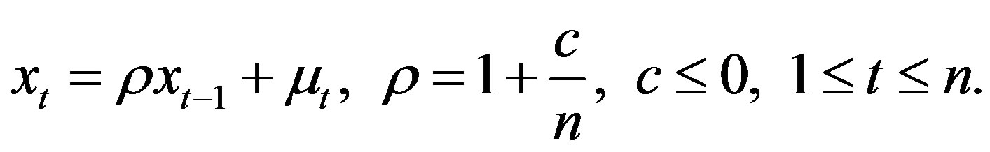
We propose a functional regression model to capture the stability of asset returns. It is well known that a nonlinear function would better to characterize dynamic relationship between the stock return and the related financial variables, the two innovations may have a time dependent nonlinear relationship, and the log dividend-price ratio , is a integrated or nearly integrated process [3, 22]. Our model runs as follows.
 (1)
(1)
 (2)
(2)
where innovation  is exogenous.
To remove the endogeneity, we project  onto
onto  by
by , which is strictly increasing in
  and
and  is uncorrelated with
  and
and . See, for example, [23] for endogenous variable. Thus the model becomes
 (3)
(3)
 (4)
(4)
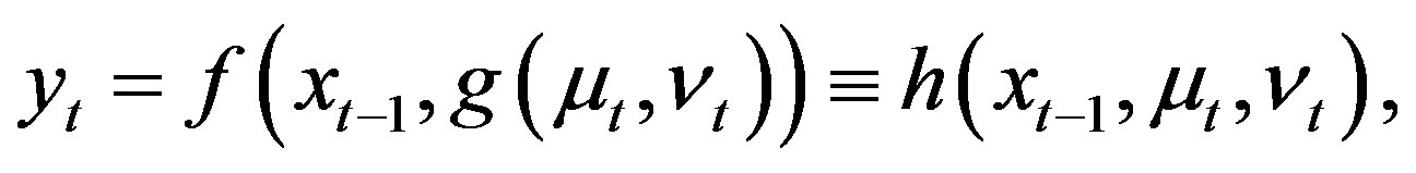
The function f can be estimated once function h is estimated due to the strict increasing of 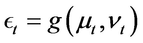 with respect to
  and the Equation (4). Indeed if the functions f and g are linear, the model reduces to [22].
3. Nonparametric Estimation
Once parametric structures are not specified for the functions h in the economic model, the function h is nonadditive in![]() . If the function is additive in unobservable random term
. If the function is additive in unobservable random term![]() , one can interpret this added unobservable random term as being a function of the observable and other unobservable variables, which is hard to estimate this function of the observable and unobservable variables. Here we estimate a nonparametric function h, not necessarily additive.
, one can interpret this added unobservable random term as being a function of the observable and other unobservable variables, which is hard to estimate this function of the observable and unobservable variables. Here we estimate a nonparametric function h, not necessarily additive.
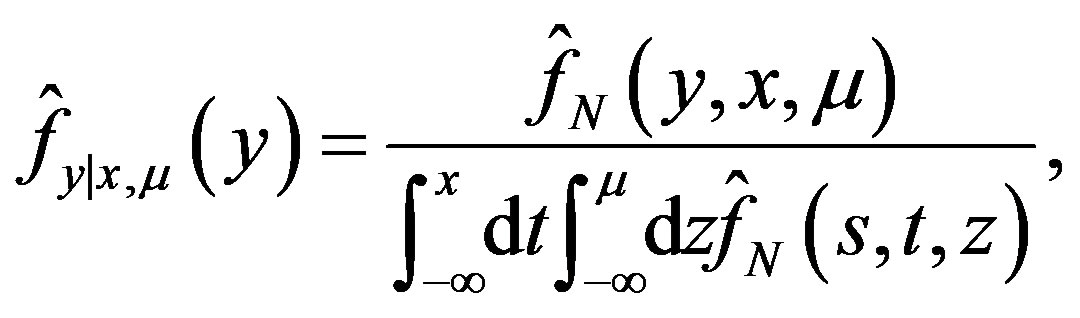
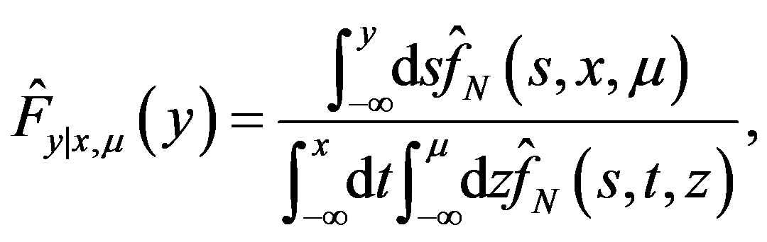
To estimate the regression function h in the basic model (3), we will derive its expression in terms of the distribution of the vector of the observable variables. Once the unknown regression function is expressed in terms of the distribution of , we will derive its nonparametric estimator for the unknown regression function by substituting the distribution of the observable variables. Though any type of nonparametric estimator for this distribution can be used, we present here the details and asymptotic properties for the case in which the conditional cumulative distributed functions are estimated by the method of kernels. To express the unknown function in terms of the distribution of the observable variables, we need the following assumptions [24].
Assumption 1  is independent of
  and
and , and
, and .
.
Assumption 2 For all values of  and
and , the function h is strictly increasing in
 .
.
Assumption 1 guarantees that the distribution of  is the same for all values of
  and
and . Assumption 2 guarantees that the distribution of
  can be obtained from the conditional distribution of
  given
given  and
and .
.
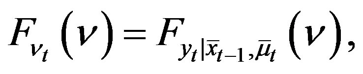
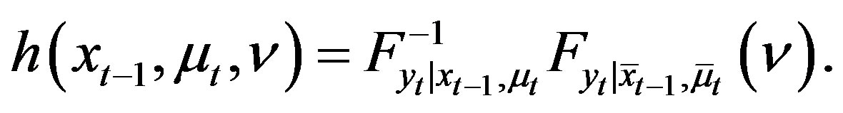
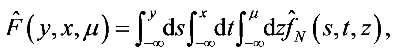
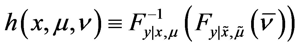
Theorem 3 Under Assumptions 1 and 2, the mapping between the unknown regression function h and , the distribution of the observable variables
  is given by
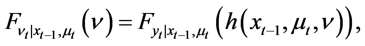 (5)
(5)
for all  with
with .
.
Proof.
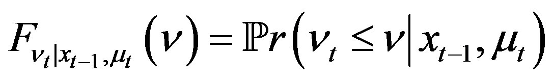 (6)
(6)
 (7)
(7)
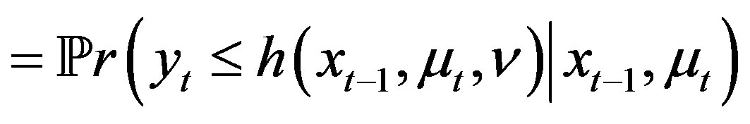 (8)
(8)
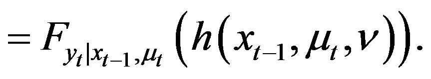 (9)
(9)
According to the theorem above, the following four cases hold. 
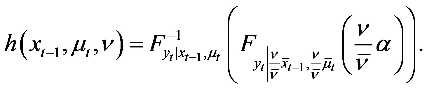
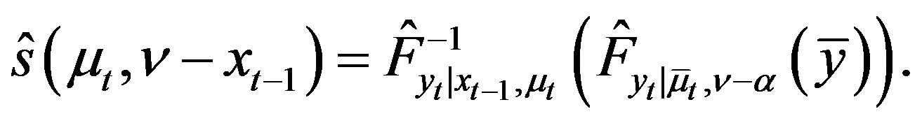
Lemma 4 (Case 1) For all  and some
  with
with ,
,
 (10)
(10)
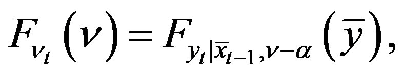
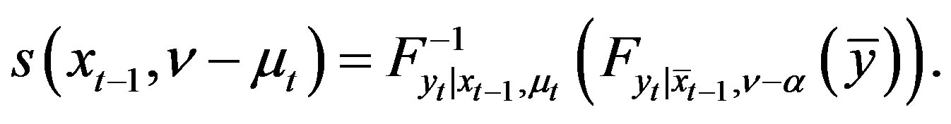
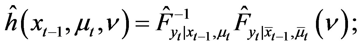
and Assumptions 1 and 2 hold. Then
 (11)
(11)
 (12)
(12)
Lemma 5 (Case 2) For all  and some
  with
with , and
, and  such that
  and
and ,
,
 (13)
(13)
 (14)
(14)
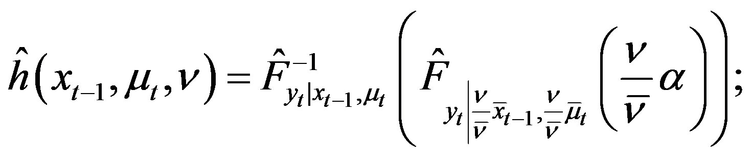
and Assumptions 1 and 2 hold. Then
 (15)
(15)
 (16)
(16)
Lemma 6 (Case 3) For some unknown function , all
, all  and some
 , some
 , and some
  such that
 , and
, and
 (17)
(17)
 (18)
(18)
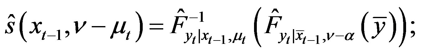
Assumptions 1 and 2 hold, and for all ,
,  is strictly increasing. Then, for
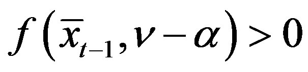 ,
,
 (19)
(19)
 (20)
(20)
Lemma 7 (Case 4) For some unknown function , all
, all  and some
 , some
 , and some
  such that
 , and
, and
 (21)
(21)
 (22)
(22)
Assumptions 1 and 2 hold, and for all ,
,  is strictly increasing. Then, for
 ,
,
 (23)
(23)
 (24)
(24)
Let ![]() denote the data,
denote the data,  and
and , respectively, the joint probability distribution function and cumulative distribution function of
 ,
,  and
and , respectively, their kernel estimators, and
  and
and  the kernel estimators of the conditional probability distribution function and cumulative distribution function of
 ![]() given
given  and
and . Then, according to [6], for all
 ,
,
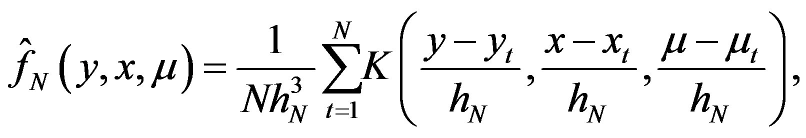 (25)
(25)
 (26)
(26)
 (27)
(27)
 (28)
(28)
where  is a kernel function and
  is the bandwidth. Hence, for case 1,
 (29)
(29)
for case 2,
 (30)
(30)
for case 3,
 (31)
(31)
for case 4,
 (32)
(32)
4. Consistency
The consistency and asymptotic normality of the estimator of the marginal or conditional distribution of  will follow from the consistency and asymptotic normality of the kernel estimator for the conditional distribution of y given x and
 . In particular, the asymptotic properties for each of the estimators for the distribution of
 ![]() given above can be derived from Theorem 13 after substituting the corresponding values of y, x, and
given above can be derived from Theorem 13 after substituting the corresponding values of y, x, and . For this result, we need following assumptions.
Assumption 8 The sequence  is independently identically distributed.
Assumption 9  has compact support
  and it is continuously differentiable on
  up to the order
  for some
 .
.
Assumption 10 The kernel function  is differentiable of order
 , the derivatives of K of order
  are Lipschitz,
  vanishes outside a compact set, integrates to 1, and is of order
  where
where .
.
Assumption 11 As  and
and ,
,  ,
,  ,
,  , and
, and 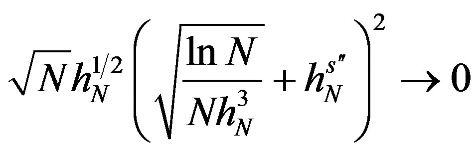 .
.
Assumption 12 .
.
Assumptions 8, 9, 10, 11 and 12 for  are similar to Assumptions
  in [24] for
 .
.
Theorem 13 Let  denote the kernel estimator for the conditional distribution of Y conditional on x and
  evaluated at
 . Assumptions 8, 9, 10, 11 and 12 hold. Then, for
  and
and ,
,
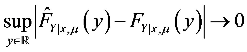 (33)
(33)
in probability, and
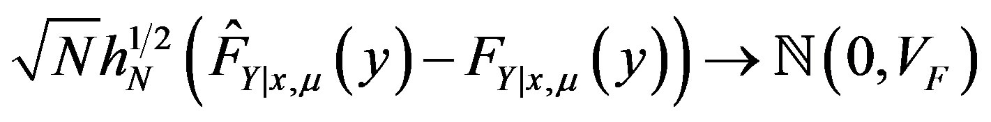 (34)
(34)
in distribution, where
 (35)
(35)
Proof. It is the case for  in the Theorem 1 in [24] in their notations when
  is not an argument.
Theorem 13 states that  converges to
  in the supremum norm, and
  is asymptotically normal with mean
  and variance equal to
 .
.
To study the asymptotic properties of the estimator for the unknown function h, notice that Equation (3), the estimator for the unknown regression function h can be obtained by substituting the true conditional distributions of Y by their kernel estimators, the consistency and asymptotic normality of the estimator of h will follow from the consistency and asymptotic normality of the functional,  , of the kernel estimator for the distribution of
 . For this result, one more assumption is required as follows.
Assumption 14 The vectors  and
and  have at least one coordinate in common, and the values
  and
and  are different at one such coordinate;
 ,
, ; and there exist
  such that
 ,
, .
.
Assumption 14 is the Assumption ![]() if
if  in their notations.
Theorem 15 Assumptions 8, 9, 10, 11 and 14 hold for  and
and . Let
. Let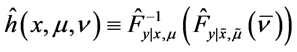 ,
, . Then,
 (36)
(36)
in probability, and
 (37)
(37)
in distribution, where
 (38)
(38)
Proof. It is the case for  of the Theorem 2 in [24] in their notations when X0 is not an argument.
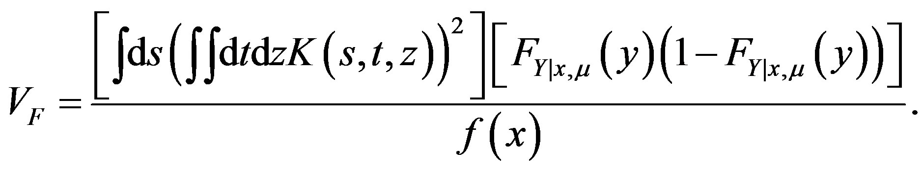
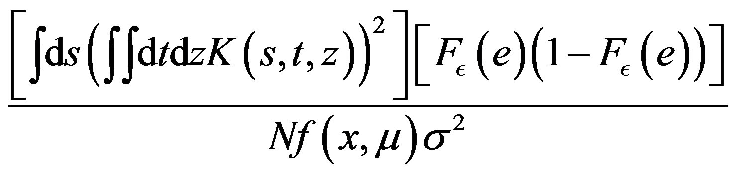
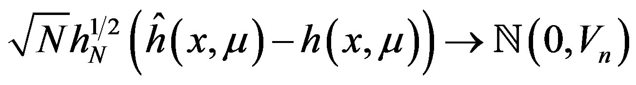
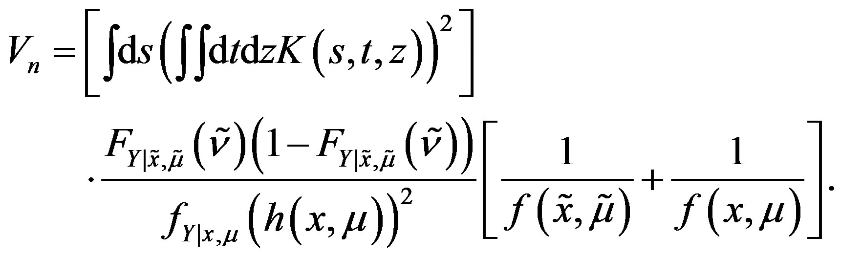
Theorem 15 implies that  is consistent and asymptotically normal with mean
  and asymptotic variance equal to
 (39)
(39)
5. Conclusions
This paper studied a predictive regression model which includes the state variable of NI(1) or I(1) and allows endogeneity, where nonlinear regression function is not necessarily additive in unobservable random terms.
We develop a nonparametric method for estimating the functional regression and find that the estimators for the distribution of the unobservable random terms and the nonparametric function are consistent and asymptotically normal. The estimators are nonlinear functionals of a kernel estimator for the distribution of the observable variables. However, the model specification or stationary is not discussed here.
More investigations are worth for the predictive application of this functional regression model due to its importance in various applications in economics and finance. For example, we here keep silent of mixing of  and
and  in the context of nonparametric functional predication, though a time-varying coefficient model is valid in [22].
6. Acknowledgement
This project was sponsored by the Scientific Research Foundation for the Returned Overseas Chinese Scholars, State Education Ministry ([2010]609), and the Science Research Foundation, Hubei Provincial Department of Education, P. R. China (D20111508) respectively.
REFERENCES
- N. G. Mankiw and M. Shapiro, “Do We Reject Too Often? Small Sample Properties of Tests of Rational Expectation models,” Economics Letters, Vol. 20, 1986, pp. 139-145.
- R. Stambaugh, “Bias in Regressions with Lagged Stochastic Regressors,” Working Paper, University of Chicago, 1986.
- J. Campbell and M. Yogo, “Efficient Tests of Stock Return Predictability,” Journal of Financial Econometrics, Vol. 81, No. 1, 2006, pp. 27-60. doi:10.1016/j.jfineco.2005.05.008
- B. S. Paye and A. Timmermann, “Instability of Return Prediction Models,” Journal of Empirical Finance, Vol. 13, No. 3, 2006, pp. 274-315. doi:10.1016/j.jempfin.2005.11.001
- T. Dangl and M. Halling, “Predictive Regressions with Time-Varying Coefficients,” Working Paper, School of Business, University of Utah, 2007.
- E. A. Nadaraya, “Some New Estimates for Distribution Functions,” Theory of Probability & Its Applications, Vol. 9, No. 3, 1964, pp. 497-500. doi:10.1137/1109069
- L. M. Viceira, “Testing for Structural Change in the Predictability of Asset Returns,” Manuscript, Harvard University, 1997.
- Y. Amihud and C. Hurvich, “Predictive Regression: A Reduced-Bias Estimation Method,” Journal of Financial and Quantitative Analysis, Vol. 39, No. 4, 2004, pp. 813- 841. doi:10.1017/S0022109000003227
- J. Y. Park and S. B. Hahn, “Cointegrating Regressions with Time Varying Coefficients,” Econometric Theory, Vol. 15, 1999, pp. 664-703. doi:10.1017/S0266466699155026
- Y. Chang and E. Martinez-Chombo, “Electricity Demand Analysis Using Cointegration and Error-Correction Models with Time Varying Parameters: The Mexican Case,” Working Paper, Texas A. M. University, 2003.
- Z. Cai, Q. Li and J. Y. Park, “Functional-Coefficient Models for Nonstationary Time Series Data,” Journal of Econometrics, Vol. 2, 2006, pp. 101-113.
- G. Elliott and J. H. Stock, “Inference in Time Series Regression When the Order of Integration of a Regressor Is Unknown,” Econometric Theory, Vol. 10, No. 3-4, 1994, pp. 672-700. doi:10.1017/S0266466600008720
- C. L. Cavanagh, G. Elliott and J. H. Stock, “Inference in Models with Nearly Integrated Regressors,” Econometric Theory, Vol. 11, No. 5, 1995, pp. 1131-1147. doi:10.1017/S0266466600009981
- W. Torous, R. Valkanov and S. Yan, “On Predicting Stock Returns with Nearly Integrated Explanatory Variables,” Journal of Business, Vol. 77, No. 4, 2004, pp. 937- 966. doi:10.1086/422634
- C. Polk, S. Thompson and T. Vuolteenaho, “Cross-Sectional Forecasts of the Equity Premium,” Journal of Financial Economics, Vol. 81, No. 1, 2006, pp. 101-141. doi:10.1016/j.jfineco.2005.03.013
- B. Rossi, “Expectation Hypothesis Tests and Predictive Regressions at Long Horizons,” Econometrics Journal, Vol. 10, No. 3, 2007, pp. 1-26. doi:10.1111/j.1368-423X.2007.00222.x
- M. Lettau and S. Ludvigsson, “Consumption, Aggregate Wealth, and Expected Stock Returns,” Journal of Finance, Vol. 56, No. 3, 2001, pp. 815-849. doi:10.1111/0022-1082.00347
- A. Goyal and I. Welch, “Predicting the Equity Premium with Dividend Ratios, Management Science, Vol. 49, No. 5, 2003, pp. 639-654. doi:10.1287/mnsc.49.5.639.15149
- A. Ang and G. Bekaert, “Stock Return Predictability: Is It There?” Review of Financial Studies, Vol. 20, No. 3, 2007, pp. 651-707. doi:10.1093/rfs/hhl021
- C. R. Nelson and M. J. Kim, “Predictable Stock Returns: The Role of Small Sample Bias,” Journal of Finance, Vol. 48, No. 2, 1993, pp. 641-661. doi:10.1111/j.1540-6261.1993.tb04731.x
- J. Lewellen, “Predicting Returns with Financial Ratios,” Journal of Financial Economics, Vol. 74, No. 2, 2004, pp. 209-235. doi:10.1016/j.jfineco.2002.11.002
- Z. Cai and Y. Wang, “Instability of Predictability of Asset Returns,” Working Paper, University of North Carolina at Charlotte, 2009.
- A. Torgovitsky, “Identification of Nonseparable Models with General Instruments,” Working Paper, Yale University, 2011.
- R. L. Matzkin, “Nonparametric Estimation of Nonadditive Random Functions,” Econometrica, Vol. 71, No. 5, 2003, pp. 1339-1375. doi:10.1111/1468-0262.00452
NOTES
*Corresponding author.