Journal of Mathematical Finance
Vol.3 No.1(2013), Article ID:28390,7 pages DOI:10.4236/jmf.2013.31008
A Simple Method to Price Window Reset Options
Department of Finance, National Dong Hwa University, Hualien, Chinese Taipei
Email: hsiao@mail.ndhu.edu.tw
Received November 16, 2012; revised December 29, 2012; accepted January 11, 2013
Keywords: Window Reset Option; Black-Scholes PDE; Boundary Integral Method; Green’s Function
ABSTRACT
A window reset option is a kind of reset options with continuous reset constraints. The issue is very important for applying to employee stock options in finance or reservation options on truck-only toll lanes in traffic management. Our contribution of this study is that we proposed an accurate and simple method to price window reset options. The option price is formulated as the solution of a boundary value problem of the Black-Scholes PDE. The problem is then transformed into an initial-boundary value problem of the heat equation. Then Green’s function is applied to solve the heat equation problem. Finally, the option price is calculated numerically. A numerical example and some discussions are presented in this paper.
1. Introduction
A reset option is a path-dependent derivative whose payoff depends on the historical prices of underlying assets. The strike price can be adjusted according to pre-specified conditions during the specified discrete monitoring dates or a continuous period. The main function of the reset clause is to protect investors from downside risk that affects the underlying prices during bear or uncertain financial markets.
A window reset option is a reset option with a continuous reset period which is called the reset window. The strike price of a window reset option is reset to a prespecified level provided the underlying asset price being below the reset threshold during the pre-specified window period. This study presents a simple and effective method for pricing window reset options under BlackScholes economy assumptions.
Derivatives with reset clauses are extremely popular. For example, the Chicago Board Options Exchange (CBOE) and the New York Stock Exchange (NYSE) traded the S&P 500 index put warrants with a threemonth reset period in 1996. In June 1997, Morgan Stanley issued a warrant containing a reset clause on the Hong Kong stock market [1]. Furthermore, Grand Cathay Securities issued six American-style reset warrants listed on the Taiwan Stock Exchange from 1998 to 1999, all of which were multiple reset warrants that possessed multiple reset prices during the reset period.
Since Black and Scholes [2] and Merton [3] developed the option valuation formula, the Black-Scholes model has become the mainstream framework for option pricing. Most researchers have proposed various pricing methods for the valuation of reset options with discrete monitoring dates. Gray and Whaley [4,5] studied the S&P 500 index reset put warrant and obtained a closed-form solution for a reset warrant with a single reset date. Cheng and Zhang [1] evaluated a reset option with multiple discrete reset dates. They obtained a closed-form solution by using probability method. Liao and Wang [6] built on the work of Cheng and Zhang [1] and used multiple normal distribution functions to price a reset option. Dai, Fang and Lyuu [7] studied the analytics for geometric average trigger reset options. Hsiao, Wang and Chen [8] priced an arithmetic average reset option using the Green function method.
In recent years, it became more and more popular for companies to issue employee stock options with reset constraints on a lock-up period. When the employee stock option is embedded with a continuous reset period, it is called the window reset option. However, there are few studies about pricing continuous reset options since there is no closed-form exact solution for the valuation of window reset options. Liao and Wang [6] formulated the price of a continuous reset option to be equal to the difference between the prices of a down-and-out barrier option with an original strike price and a down-and-in barrier option with a reset strike price. Their method can’t solve the valuation of window reset options, since the method is useful only when the end of reset date is the maturity of the contract.
Our contribution of this study is that we proposed an accurate and simple method to formulate window reset option as the solution to a boundary value problem of the Black-Scholes PDE. The problem was simplified into an initial-boundary value problem of a heat equation. The solution could be represented explicitly via a boundary integral representation [9]. Additionally, if we change the reset clauses to a barrier condition, the method can also apply to solve window barrier options [10]. Finally, the numerical integration is employed to calculate the option price. An example of a window reset option is presented to demonstrate the influence of different levels of stock volatility on option prices.
The rest of this paper is organized as follows. The window reset option is detailed in Section 2. In Section 3, we formulate the mathematical model, while in Section 4, we transform it into a boundary value problem of the heat equation. The boundary integral representation of the solution is then obtained. Next, in Section 5 we present a numerical example. Finally, in the last section there are conclusions and discussions.
2. Window Reset Options
A window reset option is a reset option with a partial continuous reset window. The strike price of a window reset option is reset to a new level if the price of underlying asset is below the threshold at a pre-specific period. This period is called the reset window. The path of stock value will determine the strike price of the option. In this article, the period, the strike price and the reset level are denoted by , E and
  respectively. The reset price is assumed to be the same as the reset level. Therefore, at expiration T, the option price C(s,T) is
 (1)
(1)
where 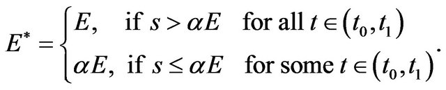
3. Mathematical Model
In this section, we establish the mathematical model for a window reset option. Under the Black-Scholes [2] economy assumptions, when the stock price, s, follows a geometric Brown motion, the price of the option, C, must satisfy the Black-Scholes PDE as follows:
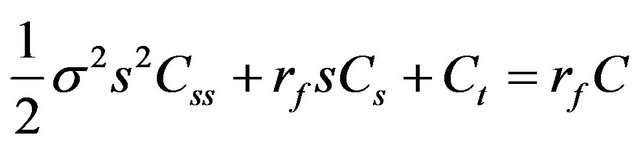 (2)
(2)
where  is the stock’s volatility, rf is the risk-free interest rate, and t is the time.
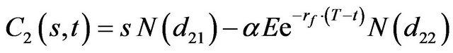
At the end of the reset window, the strike price is determined. Thus, by the Black-Scholes formula, the price has to be
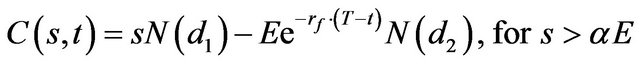 (3)
(3)
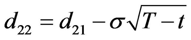
where N(.) is the standard normal cumulative distribution function,
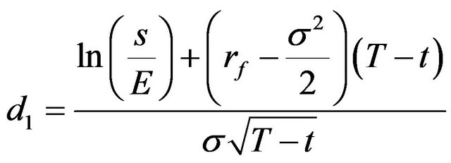 ,
, .
.
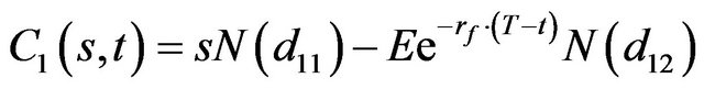
Let C1(s,t) denote the option price with strike E and C2(s,t) with strike . Then the formulae for C1(s,t) and C2(s,t) are as follows:
 (4)
(4)
where ,
,
 .
.
 (5)
(5)
where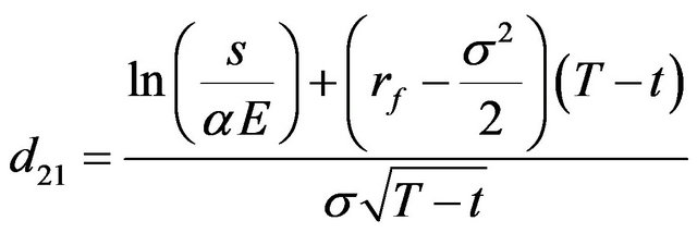 ,
,
 .
.
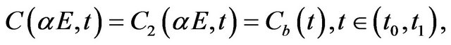
During the reset window, if the stock price has touched the reset level, the strike price is reset to  and never changes until expiration. In this situation, the option price can be expressed by the Black-Scholes formula, i.e. C(s,t) = C2(s,t). Thus, we only need to evaluate the option price C(s,t) before the stock price touches the reset level during the window. The option price C(s,t) fulfills the Black-Sholes Equation (2). When the stock price touches the reset level, the price C(s,t) = C2(s,t) . If the stock prices do not touch the reset level through the window, at the end of the window, the price has to be C1(s,t). Therefore
 (6)
(6)
and
 (7)
(7)
In the domain of  and
and . Equation (2) is the PDE, Formula (6) is the boundary condition and Formula (7) is the initial condition.
4. Variables Transformation and Integral Representation
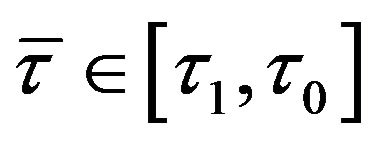
In this section, we employ a variables transformation to simplify the boundary value problem established in the last section. After the variables transformation as in Equation (8), the Black -Scholes PDE will be simplified into the homogeneous heat equation as Equation (9), and the time variables, t0, t1, and T will be transformed into time to maturity as ,
,  , and 0.
Let
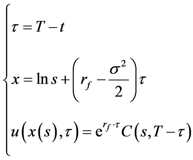 (8)
(8)
The Black-Scholes PDE becomes
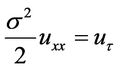 (9)
(9)
The boundary condition becomes:
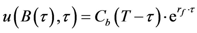 where
where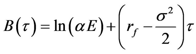 ,
, .
.
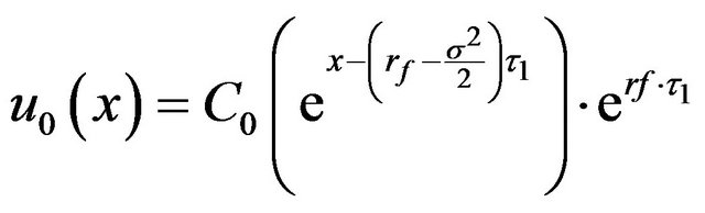
The initial condition becomes
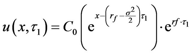 , for
, for
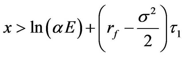 .
.
The transformed boundary value problem is an initialboundary value problem of the heat equation. The solution to the problem can be represented by Shen and Wang [9].
Let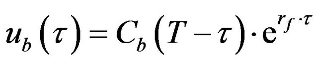 ,
,
 and
and
 .
.
 (10)
(10)
where ,
, .
.
The function G(.) is a fundamental solution of the heat equation. The formula (10) is called the integral representation of the heat equation. There exists a fundamental solution G such that G is banished on the boundary , i.e.
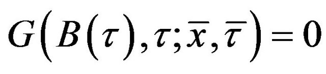 . The fundamental solution G is called Green’s function with boundary
 .
.
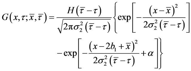 (11)
(11)
where b1 is the transformed reset threshold at ,
,
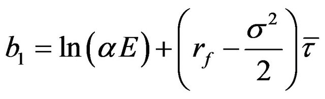 ,
,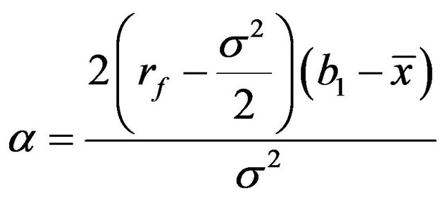 .
.
 is the Heaviside step function and is defined in Equation (12).
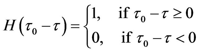 (12)
(12)
The partial derivative of the Green function about the variable x is as follows.
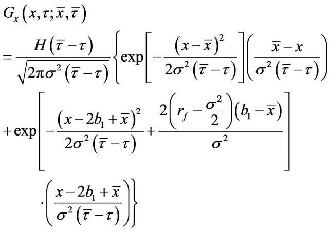 (13)
(13)
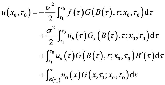
When we use the characteristics of the Green function at the boundary condition, we can further simplify the integral representation (10) to equation (14). Therefore, we substitute Green’s function with boundary into the integral representation (10), and the integral representation is as follows.
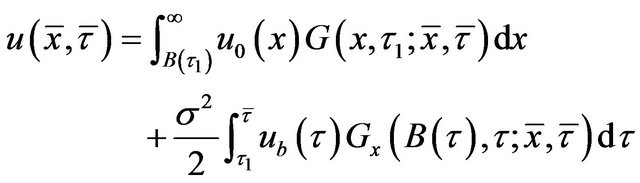 (14)
(14)
where ,
,  , and
, and
 . The solution u is expressed explicitly in formula (14).
The first term of Equation (14) is the contribution of initial data, and it can be calculated easily via Simpson’s rule. The second term of Equation (14) is the contribution of boundary data, and we use the Gaussian quadrature1, which is a simile accurate method to approach the solution of the integration, to calculate it as follows:
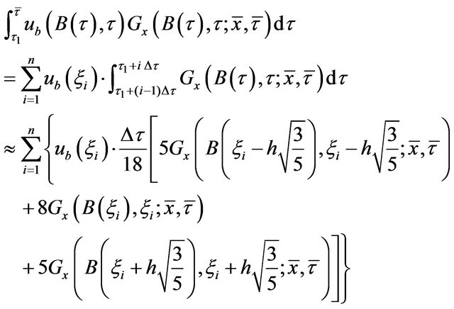
(15)
where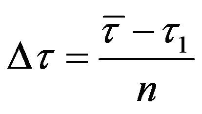 ,
, 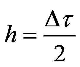 ,
,  ,
, .
.
Thus, we obtain the transformed valuation of window reset option, . The option price is
 (16)
(16)
where  and
and .
.
5. Numerical Example
Considering a window reset option, the original strike price E = 100, the reset rate , the risk-free rate rf = 0.02. Option life begins at time t0. The reset period is the interval [t0, t1], t1 = t0 + 0.25 year. The time to maturity of the contract is T = t0 + 1 year. The accuracy, calculation time and numerical orders of option price with respect to the volatilities 0.25, 0.5 and 0.75 are showed in Table 1-3. The integration results would be accurate at least to the fourth decimal place in all tables. If we double the partition numbers, the calculation time increases around four folds. It shows that our method is useful to price the window reset option.
On the other hand, we compare the valuation of window reset option with different volatility to vanilla option in Figures 1-3. The value of a window reset option increases with the current stock price. Figure 4 presents the differences between the value of a vanilla option and a window reset option with stock volatility 0.25, 0.5, 0.75 respectively. We can tell that the difference is significant when the volatility of stock price is at a low level and the current stock price is close to the reset threshold , 90. When the volatility of stock price is low, the difference curve varies violently and decreases quickly to zero in Figure 4.
Table 1. The accuracy of the option pricing with the volatility 0.25.
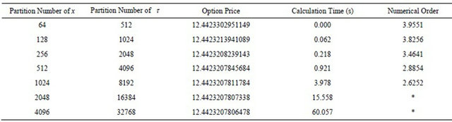
Note: The current stock price S0 = 100, the original strike price E = 100; the reset rate α = 90%; the risk-free rate rf = 0.02; option life begins at time t0; the reset window is from t0 to t1 = t0 + 0.25; time to maturity T = t0 + 1.
Table 2. The accuracy of the option pricing with the volatility 0.5.
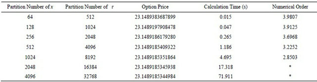
Note: The current stock price S0 = 100, the original strike price E = 100; the reset rate α = 90%; the risk-free rate rf = 0.02; option life begins at time t0; the reset window is from t0 to t1 = t0 + 0.25; time to maturity T = t0 + 1.
Table 3. The accuracy of the option pricing with the volatility 0.75.
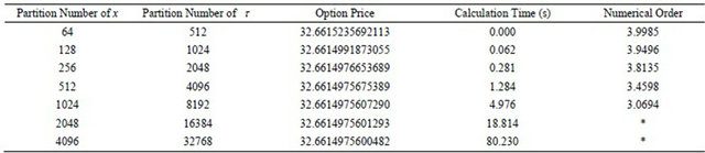
Note: the current stock price S0 = 100, the original strike price E = 100; the reset rate α = 90%; the risk-free rate rf = 0.02; option life begins at time t0; the reset window is from t0 to t1 = t0 + 0.25; time to maturity T = t0 + 1.
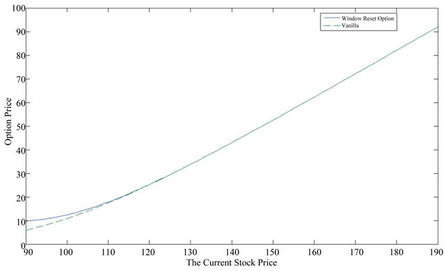
Figure 1. The valuation of a vanilla option and window reset option with a stock volatility 0.25 under different stock prices. Note: The original strike price E = 100; the reset rate α = 90%; the risk-free rate rf = 0.02; option life begins at time t0; the reset window is from t0 to t1 = t0 + 0.25; time to maturity T = t0 + 1.
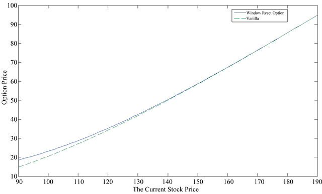
Figure 2. The valuation of the vanilla option and window reset option with a stock volatility 0.5 under different stock prices. Note: The original strike price E = 100; the reset rate α = 90%; the risk-free rate rf = 0.02; option life begins at time t0; the reset window is from t0 to t1 = t0 + 0.25; time to maturity T = t0 + 1.

Figure 3. The valuation of the vanilla option and window reset option with a stock volatility 0.75 under different stock prices. Note: the original strike price E = 100; the reset rate α = 90%; the risk-free rate rf = 0.02; option life begins at time t0; the reset window is from t0 to t1 = t0 + 0.25; time to maturity T = t0 + 1.
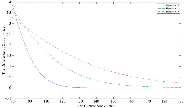
Figure 4. The difference between a vanilla option and window reset option with stock volatility 0.25, 0.5, 0.75 under different stock prices. Note: the original strike price E = 100; the reset rate α = 90%; the risk-free rate rf = 0.02; option life begins at time t0; the reset window is from t0 to t1 = t0 + 0.25; time to maturity T = t0 + 1.
6. Conclusions and Discussions
Emerging derivatives are more and more popular in recent years. In this paper, we focus on the valuation of a window reset option which is a kind of reset options with continuous reset constraints. The issue is very important for applying to employee stock options in finance or reservation options on truck-only toll lanes in traffic management. Our contribution of this study is that we proposed an accurate and simple method to price window reset options. We use the efficient integral representation of PDE to present the valuation of window reset option and use the numerical method, Simpson’s rule and Gauss integral method, to calculate it.
Our pricing method is useful to obtain accurate numerical results fast. The difference between a vanilla option and a window reset option is significant when the stock volatility is at a low level and the current stock price is close to the reset threshold. In our numerical example, when the current stock price is about more than twofolds standard deviations, the price of window reset option is close to the value of vanilla option. The numerical result is related to the reset period and the volatility of stock price, since a short reset period or a low level of stock volatility will decrease the effect of the reset constraints. Therefore, the price difference volatilizes when the stock volatility is at a low level as shown in Figure 4.
REFERENCES
- W. Cheng and S. Zhang, “The Analytics of Reset Options,” Journal of Derivatives, Vol. 8, No. 1, 2000, pp. 59-71. doi:10.3905/jod.2000.319114
- F. Black and M. Scholes, “The Pricing of Options and Corporate Liabilities,” The Journal of Political Economy, Vol. 81, No. 3, 1973, pp. 637-654. doi:10.1086/260062
- R. C. Merton, “Theory of Rational Option Pricing,” Bell Journal of Economics and Management Science, Vol. 4, No. 1, 1973, pp. 141-183. doi:10.2307/3003143
- S. Gray and R. Whaley, “Valuing S&P 500 Bear Market Reset Warrants with A Periodic Reset,” Journal of Derivatives, Vol. 5, No. 1, 1997, pp. 99-106. doi:10.3905/jod.1997.407987
- S. Gray and R. Whaley, “Reset Put Options: Valuation, Risk Characteristics, and an Application,” Australian Journal of Management, Vol. 24, No. 1, 1999, pp. 1-20. doi:10.1177/031289629902400101
- S.-L. Liao and C.-W. Wang, “The Valuation of Reset Options with Multiple Strike Resets and Reset Dates,” The Journal of Futures and Markets, Vol. 23, No. 1, 2003, pp. 87-107. doi:10.1002/fut.10055
- T. S. Dai, Y. Y. Fang and Y. D. Lyuu, “Analytics for Geometric Average Trigger Reset Options,” Applied Economics Letters, Vol. 12, No. 13, 2005, pp. 835-840. doi:10.1080/1350485052000345500
- Y. L. Hsiao, A. M. L. Wang and C. Y. Chen, “Pricing an Arithmetic Average Reset Option Using the Green Function Method,” Asia Pacific Management Review, 2011.
- S. Y. Shen and A. M. L. Wang, “On Stop-Loss Strategies for Stock Investments,” Applied Mathematics and Computation, Vol. 119, No. 2-3, 2001, pp. 317-337. doi:10.1016/S0096-3003(99)00229-5
- Y.-L. Hsiao, “Closed-Form Approximate Solutions of Window Barrier Options with Term-Structure Volatility and Interest Rates Using the Boundary Integral Method,” Journal of Mathematical Finance, Vol. 2, No. 4, 2012, pp. 291-302. doi:10.4236/jmf.2012.24032
- D. Kincaid and W. Chency, “Numerical Analysis,” Brooks/ Code Publishing Company, Pacific Grove, 1991, p. 460.
NOTES
1David Kincaid and Ward Chency [11], “Numerical Analysis,” Brooks/ Code Publishing Company, Pacific Grove, p. 460.