Open Journal of Statistics
Vol.2 No.5(2012), Article ID:25550,7 pages DOI:10.4236/ojs.2012.25066
Spike-and-Slab Dirichlet Process Mixture Models
1Department of Statistical Science, Duke University, Durham, USA
2School of Science and Information, Qingdao Agricultural University, Qingdao, China
Email: kc52@stat.duke.edu, wshcui@qau.edu.cn
Received October 16, 2012; revised November 18, 2012; accepted November 30, 2012
Keywords: Spike and Slab; Dirichlet Process; Bayesian Expectation-Maximization (BEM); Mixture
ABSTRACT
In this paper, Spike-and-Slab Dirichlet Process (SS-DP) priors are introduced and discussed for non-parametric Bayesian modeling and inference, especially in the mixture models context. Specifying a spike-and-slab base measure for DP priors combines the merits of Dirichlet process and spike-and-slab priors and serves as a flexible approach in Bayesian model selection and averaging. Computationally, Bayesian Expectation Maximization (BEM) is utilized to obtain MAP estimates. Two simulated examples in mixture modeling and time series analysis contexts demonstrate the models and computational methodology.
1. Introduction
Dirichlet Process (DP) priors are used across a wide variety of applications of Bayesian analysis, including Bayesian model validation, density estimation and mixture modeling. Specifically in hierarchical mixture models, the nonparametric nature of the Dirichlet process translates to mixture models with a countably infinite number of components and is used to specify latent patterns of heterogeneity. It allows for uncertainty about the number of mixture components and component specific parameters.
On the other hand, if the typical Dirichlet process prior with a continuous base measure  is used as the prior for the distribution of parameter
 , this requires a known parametric model and fixed parameter space. However, this is often not the case. For example, in mixture models, we often deal with cases with model uncertainty where the parameter space of one mixture component might be smaller than that of another. In these cases, a DP priors with continuous base measure are both theoretically and philosophically not right to use. Instead, we want to further integrate model selection techniques into the model to allow for more flexibility.
Bayesian spike-and-slab approaches to parameter selection have been proposed [1,2], and used as prior distributions in the Bayesian model selection and averaging literature [3]. Spike-and-slab distributions are mixtures of two distributions: the spike refers to a point mass distribution (say, at zero) and the other distribution is a continuous distribution for the parameter if it is not zero. Recently, the use of spike-and-slab distribution combined with Dirichlet process prior has been proposed in multiple hypothesis testing [4,5]. This approach is shown to readily accommodate sharp hypothesis, which cannot be tested using regular Dirichlet process with continuous base measure (due to the fact that sharp hypotheses will have zero posterior probability) [6].
In this study, we propose the use of Spike-and-Slab Dirichlet process (SS-DP) priors, especially in mixture models. The uncertainty about model and parameter space is incorporated in the model by modeling the unknown distributions of parameters with SS-DP priors which allow degeneration of certain parameters. We show that SS-DP mixture models are flexible models allowing both unknown number of components and different component-specific parameter spaces.
2. Models and Methods
2.1. Spike-and-Slab Dirichlet Process Mixture Models
Consider a Dirichlet Process Mixture (DPM) model with infinite number of components of the form
 . Hence, y is distributed as a mixture of distributions with the same parametric form f and parameter space, but different parameter values. Assuming that all the parameters
 ![]() are from the continues distribution G, the mixture model can be expressed hierarchically as a DPM model of the form:
are from the continues distribution G, the mixture model can be expressed hierarchically as a DPM model of the form:
 (1)
(1)
where  is the Dirichlet Process with continuous base measure
  and spread
  [7,8], and G is a random distribution drawn from the Dirichlet process.
The SS-DP mixture model we proposed here is an extension of the DPM model, which allows different parameter spaces of f, especially with some of the parameters degenerated. This flexibility is achieved by letting the base measure  be spike-and-slab with a mixture of point mass (typically at 0) and the other (continuous) distribution instead.
Hence, the SS-DP mixture Model is:
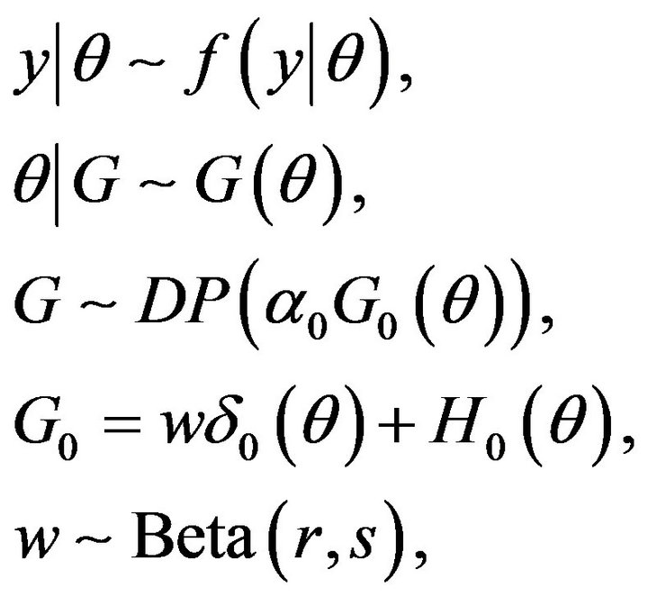 (2)
(2)
where  is a Dirac delta function,
  is a continuous measure and w is the mixing weight with a Beta prior distribution.
Clearly, by allowing the values of parameters to be exactly 0, SS-DP mixture models simultaneously incorporate the uncertainty of component-specific parameter space. It is worth noting that in many applications, this degeneration of specific parameter(s) (or an exact value of a parameter) defines important regime switching or phase change that cannot be modeled by traditional DPM models with continuous base measure. Examples of such cases are shown in the simulation study section.
2.2. Truncated SS-DP Mixture Models
In practice, for problems that require unknown number of mixture components and uncertainty of component-specific parameter space, we can use the stick-breaking representation of Dirichlet process [9] to truncate the SS-DP mixture models at a maximum number of components J. To illustrate, the following example of truncated SS-DP mixture models is shown, which will also be the basic model for our simulation studies.
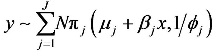
Assume that y is distributed as a mixture of K normal distributions, and the component means are linear combinations of covariates x0 and x1, where the regression coefficients of x0 may be zero in some mixture components. With the number of components K unknown, we model y as coming from a normal mixture with maximum number of components J :
:
 .
.
Furthermore, to model the possible degeneration of , SS-DP priors with a mixture of point mass at 0 and a normal distribution are placed for
 , while typical DP priors with normal base measures are used for
 , as described in (1) and (2).
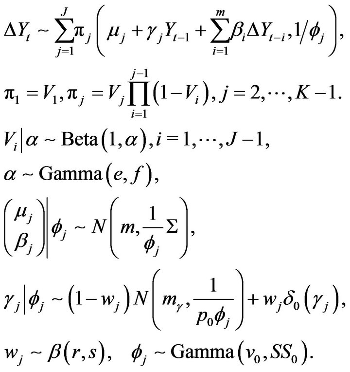
The model and priors can be written under stickbreaking representation [9] as follows:
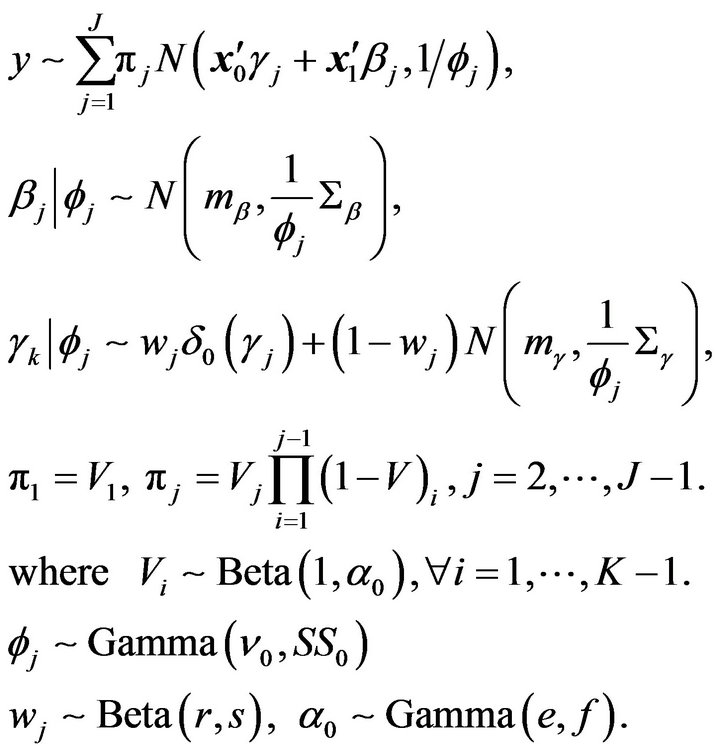 (3)
(3)
Given the model and priors, Bayesian posterior analysis of parameters provides inference of both model parameters and model uncertainty.
3. Computational Methods
For inference and posterior analysis, we propose to use Bayesian Expectation Maximization (BEM) to obtain Maximum A Posteriori (MAP) estimates of all the parameters. To help BEM visit the (local) maximum of the regions with high mass, Markov Chain Monte Carlo (MCMC) will be conducted before BEM, and multiple starting points of BEM will be chosen from MCMC samples. In comparison, label switching is expected to be a concern to interpret the MCMC results if instead Gibbs sampler is used, which is not a recommended computational method. The details of BEM are shown as follows:
Let  denote the latent component indicators, where
  if observation
  is from the
  component. And let
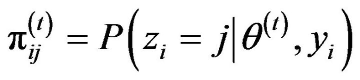
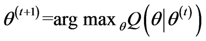
 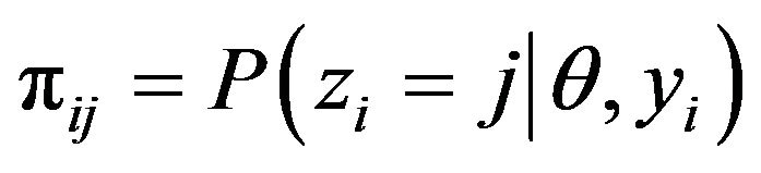 denote the assignment probability. Then the BEM is to maximize the posterior log likelihood, and iterated between the two steps:
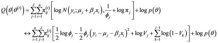
E-step: Calculate
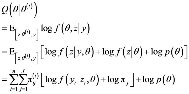
where  denotes all the parameters,
  is the parameter learning at the
  iteration,
 and
and  is the joint prior distribution of parameters.
M-step: Find the  which maximizes
 :
:
 .
.
The derivations of the M-steps given our SS-DP mixture models and priors shown in (3) are listed in detail in Appendix.
4. Simulation Study for SS-DP Mixture Model
Data are generated from a mixture of 3 normal distributions 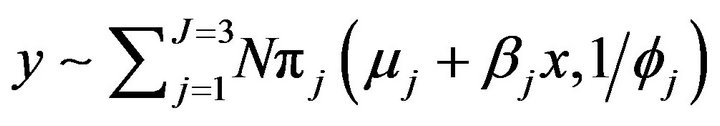 as follows, where the component mean is independent of x in one of the components.

We assume that the number of normal components are unknown a priori and set the maximum number of components J to be 20. Models and priors are used as shown in (3) and MAP estimates of all unknown quantities are obtained using BEM. Several aspects of posterior inference are checked to gauge the performance of the model and algorithms:
The MAP estimates of the model give 4 mixture components, the parameters of which are shown in Table 1. Components 1-3 recover the three components of the simulated data very well. Zero  of the third component is also inferred exactly. The model identifies one additional trivial (1.2%) fourth component. The inference of one more number of components is due to the fact that we obtained the maximum likelihood point estimate, which shows small deviation from the true number of components.
Further if we do model-based clustering based on the posterior probability of data belonging to a specific component, the classification results are shown in Figure 1, which show great similarity with the simulated components.
5. Cointegrated Time Series Analysis via SS-DP Mixture Models
One of the motivating applications for this paper arises in time series analysis where there is likely to be regime switching between a mixture of multiple stationary and non-stationary states, while the number of the states is unknown. In practice, statistical arbitragers can take advantage of the separation of regime-specific information, one of the examples of which is pair trading [10], a
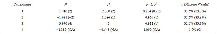
Table 1. MAP estimates of parameters via SS-DP mixture model. The estimates compared to the true values (shown in parentheses) show good inference.
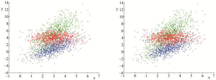
Figure 1. Model-based posterior clustering of the data compared with true clustering. The left figure shows the true 3 components of the simulated data, the right one shows the model-based clustered data into the 4 components identified using SS-DP mixture models, represented by different colors.
popular yet simple short-term speculation strategy.
The idea is of pair trading that: find two securities whose prices have been historically moving “together”. So when the spread between them widens, we short the winner and buy the loser. And if we believe that the history would repeat itself, prices will converge again and the arbitrager will profit. This “moving-together” relationship between two time series is called co-integration. Mathematically, if two time series  and
and  are co-integrated, then there exists a number k, such that
  is a stationary time series.
However, although there have been many statistical studies to find co-integrated time series, it is sometimes very hard to find such co-integrating relationship, one main reason of which is the existence of structural breaks or regime switching. In an attempt to solve the problem, we propose to use the SS-DP mixture models for modeling possible regime-switching in co-integrated time series analysis, which allows the co-integration relationship to be switched on and off between multiple regimes.
5.1. Error Correction Model and Cointegration
Suppose we have two I(1) stationary time series  and
and , and
, and 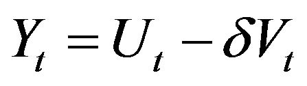 (
(![]() is known, typically people propose a
is known, typically people propose a ![]() and then test the stationary property of
and then test the stationary property of![]() ). If Y is I(0) stationary, then we say time series
). If Y is I(0) stationary, then we say time series  and
and  are co-integrated.
The way to test if ![]() is I(0) stationary is using the full Error Correction Model (ECM), which is to test the linear model:
is I(0) stationary is using the full Error Correction Model (ECM), which is to test the linear model:
 .
.
Then the ECM model tells that the time series ![]() is non-stationary if and only if
is non-stationary if and only if .
.
Given our motivation that the time series is likely to switch between a mixture of multiple stationary and nonstationary regimes, while the possible number of regimes are a priori unknown, SS-DP mixture model combined with the ECM model (SS-DP ECM mixture model) is a perfect tool here to explore the regime switching and regime-specific parameters. Also, posterior inference of  at 0 for a specific regime has the straightforward interpretation that the time series is non-stationary within the regime.
5.2. Simulated Cointegration Analysis
To testify the performance of SS-DP ECM mixture model for cointegrated time series analysis, a mixture of stationary and non-stationary time series is constructed, which switches between two stationary AR(2) processes and one non-stationary AR(2) process. We assume that the number of components are a priori unknown. And this time series mimics the tmies series generated by a co-integrated pair.
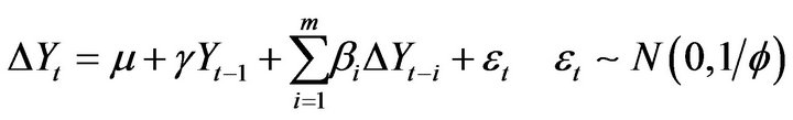
The two stationary AR(2) model and one non-stationary AR(2) model, and their corresponding Error Correction Model (ECM) are shown (the (non-)stationary property can be easily tested by the unit root test [11]):
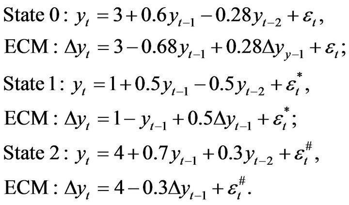
The simulated time series of length 300 is shown in Figure 2, with the probability of simulating from the three states being ,
,  and
and  respectively.
We applied SS-DP mixture model combined with the ECM model to model the regime-switching time series as a mixture of statioanry and non-stationary time series. The model and stick-breaking representation of the SS-DP priors are shown as follows:
We set maximum number of components J to be truncated at 20 and used BEM to obtain MAP estimates of all unknown quantities. The results show correct identification of 3 mixture components (regimes). Since in most cases we are especially interested in identifying and excluding time points in the non-stationary regime, Figure 2 shows that the posterior inferred non-stationary time points (green dots) recover the true non-stationary time points (red dots) well. Good MAP estimates of the regime-specific parameters  are also obtained as shown in Table 2.
5.3. Model-Based Decision Making
SS-DP mixture models are especially important in this case, because the characterization of stationary regime is
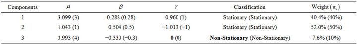
Table 2. MAP estimates of SS-DP ECM mixture models for the regime-switching time series analysis. MAP estimates are compared to the true values (shown in parentheses) and show good inference.
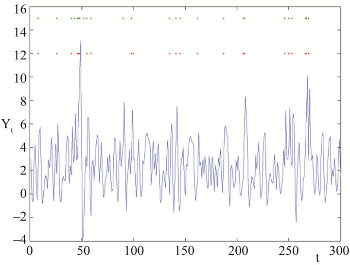
Figure 2. Characterization of non-stationary states via SS-DP ECM mixture models. The simulated time series Yt is shown. The red dots mark the true time points when the time series is in the non-stationary regime, and the green dots are inferred time points at which Yt is in the nonstationary regime from SS-DP ECM mixture model.
the key for decision making. To illustrate this, we use the pair trading context, in which only if the time series ![]() generated by the pair of
generated by the pair of  and
and  is in stationary regime, can people do pair trading based on the traditional rule that you open a long-short position when the pair prices have diverged by more than two historical standard deviations. And you unwind the position when it returns to historical mean. Otherwise, if
 ![]() is within the non-stationary regime at a specific time point, no action should be taken.
is within the non-stationary regime at a specific time point, no action should be taken.
Compared to the traditional co-integration test, SS-DP ECM mixture model helps make more reasonable decision, since it is only based on selected stationary regimes. In comparison, the traditional co-integration tests can only test the whole time series, which in most cases are blindly pooled data consisting of both stationary and non-stationary states.
6. Concluding Remarks
In this paper, we introduced and studied spike-and-slab Dirichlet process priors, especially in the mixture models framework, which add more flexibility to the traditional nonparametric mixture models by allowing uncertainty about the component-specific parameter space. Given the wide use of mixture models in a variety of fields including biological science, machine learning, econometrics and finance, more flexible while computationally efficient models are definitely worth exploring.
REFERENCES
- J. F. Geweke, “Variable Selection and Model Comparison in Regression,” Working Papers 539, Federal Reserve Bank of Minneapolis, Minneapolis, 1994.
- T. J. Mitchell and J. J. Beauchamp, “Bayesian Variable Selection in Linear Regression,” Journal of the American Statistical Association, Vol. 83, No. 404, 1988, pp. 1023- 1032,
- E. I. George and R. E. McCulloch, “Variable Selection via Gibbs Sampling,” Journal of the American Statistical Association, Vol. 88, No. 423, 1993, pp. 881-889.
- D. B. Dahl and M. A. Newton, “Multiple Hypothesis Testing by Clustering Treatment Effects,” Journal of the American Statistical Association, Vol. 102, No. 478, 2007, pp. 517-526.
- D. B. Dahl, Q. Mo and M. Vannucci, “Simultaneous Inference for Multiple Testing and Clustering via a Dirichlet Process Mixture Model,” Statistical Modelling, Vol. 8, No. 1, 2008, pp. 23-29.
- S. Kim, D. B. Dahl and M. Vannucci, “Spiked Dirichlet Process Prior for Bayesian Multiple Hypothesis Testing in Random Effects Models,” Bayesian Analysis, Vol. 4, No. 4, 2009, pp. 707-732.
- T. S. Ferguson, “A Bayesian Analysis of Some NonParametric Problems,” The Annals of Statistics, Vol. 1, No. 2, 1973, pp. 209-230.
- T. S. Ferguson, “Prior Distributions on Spaces of Probability Measures,” Annals of Statistics, Vol. 2, No. 4, 1974, pp. 615-629.
- J. Sethuraman, “A Constructive Definition of Dirichlet Priors,” Statistica Sinica, Vol. 4, 1994, pp. 639-650.
- E. P. Chan, “Quantitative Trading,” John Wiley and Sons, Hoboken, 2008.
- D. A. Dickey and W. A. Fuller, “Distribution of the Estimators for Autoregressive Time Series with a Unit Root,” Journal of the American Statistical Association, Vol. 74, No. 366, 1979, pp. 427-431.
Appendix
Bayesian Expectation Maximization (BEM)
The derivations for BEM are based on the model for simulation Study 1:
and priors specified in Equation (3).
M-step for the SS-DP mixture model for simulation Study 1
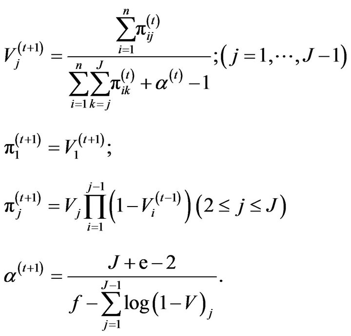
The solutions to the first-order differential equations are:
However, when we look at the first order differential equations for ,
,  ,
,  and
and , they are complicated due to the existence of delta function (not shown here). In order to find the optimal values
 ,
,  ,
,
 and
and . The following two-step trick can be applied.
1) Split into  and
and  two cases. For each case, find the values of parameters that are (local) maximum.
Note: For  case, there might be no (local) maximum that can be found (or very hard to directly confirm that a maximum is found), but we can indeed use the reference solutions provided below (
 ,
, ,
, and
and ) to continue to find the global maximum.
2) Compare the solutions of the two cases by log posterior density, the ones that give the bigger log posterior density will be set to be ,
,  ,
,  and
and .
.
Derivations for .
.
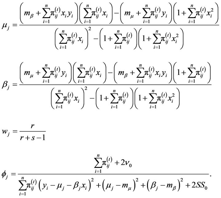
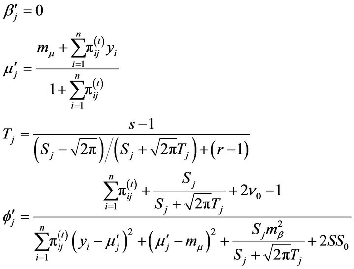
If :
:
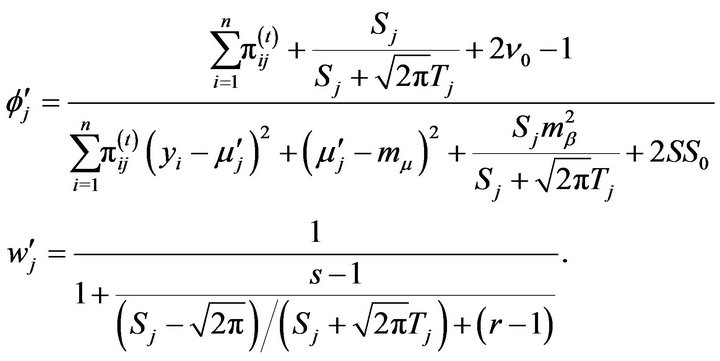
The solutions to  all have close form, which are:
If :
:
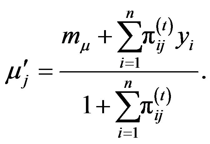
We can immediately get the solution to , which is:
For  and
and , apparently the solutions to the two equations (which are
 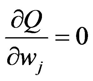 and
and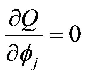 ) do not have close form. Numerical Methods will be applied to get accurate enough approximate solutions.
where
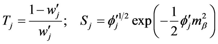 .
.
And the last two equations are used to iteratively find the approximate solution to  and
and , which are:
Compare solutions  with
with
 , the one that gives larger log posterior density is set to
 .
.
BEM for simulation Study 2 with SS-DP ECM mixture model is obtained similarly.