Abstract

In this paper, blocking in response surface for fitting first order model incorporating neighbour effects has been investigated. The conditions for orthogonal estimation of the parameters of the model have been obtained. A method of constructing designs which ensures the constancy of variance of the parameter estimates of the model has also been given.

1. Introduction

Response Surface Methodology (RSM) is used to explore the relationship between one or more response variable and a set of experimental variables or factors with an objective to optimize the response.

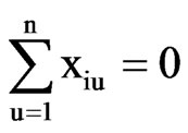
Let there be independent variables denoted by and the response variables be and there are N observations. The response is a function of input factors, i.e.

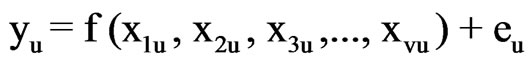
where u = 1, 2, …, N, is the level of the, (i = 1, 2, …, v) factor in the treatment combination, denotes the response obtained from treatment combination. The function f describes the form in which the response and the input variables are related and is the random error associated with the observation that is independently and normally distributed with  mean zero and common variance. For details on RSM, one may refer to Khuri and Cornell [1], Myers et al. [2].

In the literature, the work on RSM is done assuming observations to be independent and no effect of neighbouring units. However, plots in agricultural experiments are nearby and induce some overlap effects from neighbouring units. Hence, the response from a particular plot may not be the actual response from the plot but may be the joint effect of the treatment combination applied to same plot and the treatment combination applied to the neighbouring plots. For example, in an experimental trial when the combination of pesticides is used, wind drift may cause the effect of spray spill over to adjacent plots. It is thus important to study the response surface in the presence of neighbour effects which would result in more precise estimation of the parameters of the response surface model.

Draper and Guttman [3] suggested a general model for response surface problems in which it is anticipated that the response on a particular plot will be affected by overlap effects from neighbouring plots and the same has been illustrated.

Sarika et al. [4] studied second order response surface model with neighbour effects and the rotatability conditions were derived. Methods of obtaining designs satisfying the derived conditions were given.

Jaggi et al. [5] studied response surface model incorporating neighbour effects and the same has been illustrated. They showed that if the neighbour effect is present and is included in the model, there is a substantial reduction in the residual sum of squares and the response is predicted more precisely.

In response surface analysis, it is generally assumed that the experimental trials are carried out under homogeneous conditions. This assumption may not be valid in every experimental situation. In such circumstances, the experimental trials should be carried out in groups, or blocks so that the units within each block are homogeneous. Also when the number of runs is too large, it is very difficult to accommodate all the units in a single block. Blocking is usually beneficial where it is possible to identify groups, or blocks, of experimental units, such that within blocks the experimental units are considerably more homogeneous than the blocks themselves. This type of grouping makes it possible to eliminate from error variance a portion of variation attributable to block differences. The variation between the blocks in the experiment is accounted for by including block effects in the statistical model. The nature of the blocking variables has an important impact on the data analysis.

In this paper, we focus on the methodology for blocking in first order response surface model incorporating neighbour effects. The conditions for orthogonally blocked experiments for estimation of the parameters of the model and the conditions for the constancy of variance of the parameter estimates of the model are derived. Construction of response surface designs in blocks with neighbour effects has also been given and an example is discussed.

2. First Order Response Surface Methodology with Block Effects and Incorporating Neighbour Effects

2.1. Model and Estimation of Parameters

The first order response surface model with block effects can be written in the form

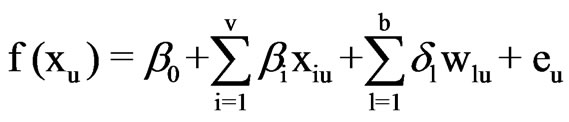, (1)

where f(x_u) denotes the observed response value at u^th experimental run, x_iu is the corresponding setting of the i^th input variable, δ_l denote the effect of the l^th block (l = 1, 2, …, b), w_lu is a dummy variable taking the value 1 if the u^th trial is carried out in the l^th block; otherwise, it is equal to zero and e_u is the random error.

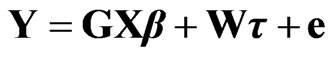
Incorporating neighbour effects to the given model, the above model with neighbour effects in matrix notation is

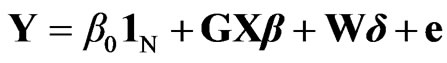(2)

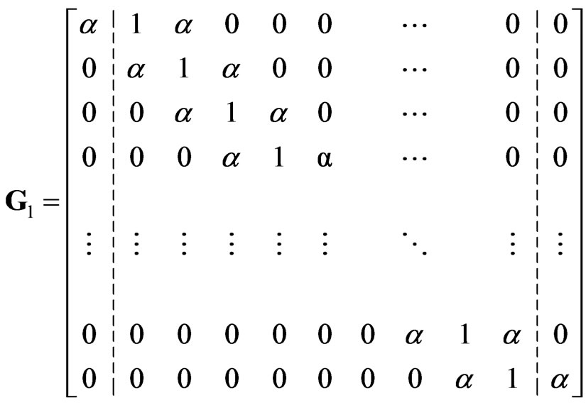
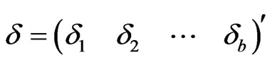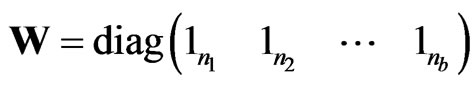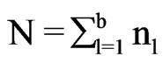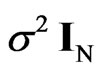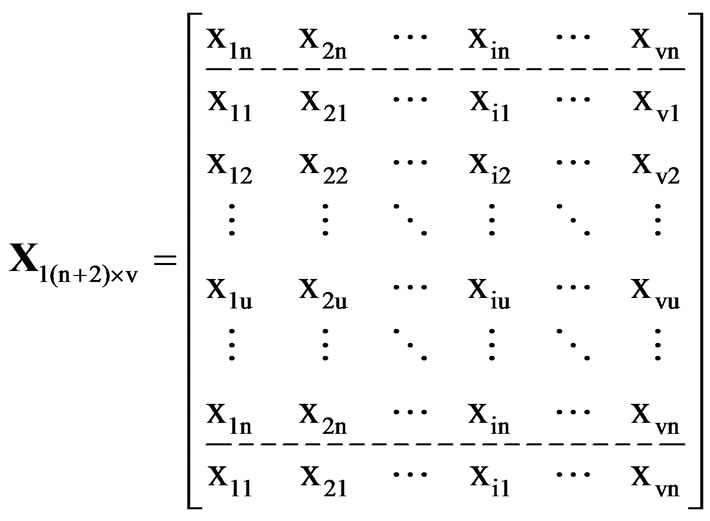
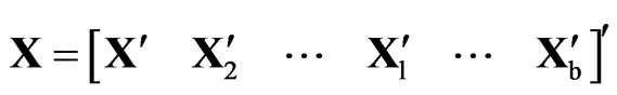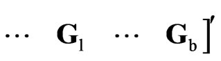
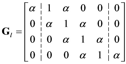
where, where δ_l denotes the effect of the l^th block (l = 1, 2, …,b) and W is a block-diagonal matrix of the form, where n_l is the size of the l^th block (l =1, 2, …, b) such that. The random error vector e is assumed to have zero mean and a variance-covariance matrix., (l = 1, 2, …, b) is a (n_l + 2) × v matrix. = ((x_iu)), i = 1, 2, …, v; u = 1, 2, …, n_l for all b blocks.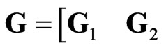, where = (l = 1, 2, …, b, s ¹ s¢ = 1, 2, …, n_l) is a n_l × (n_l + 2) neighbour matrix (assuming same neighbour structure in the b blocks) with

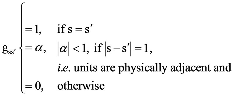(3)

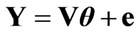
The model given in (2) is not of full column rank since the columns of W sum to 1_N. The model therefore can be written as

(4)

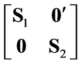
where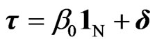. If the columns of W are linearly independent of those of GX, then model (4) is of full rank. Thus β and τ can be uniquely estimated by the method of ordinary least squares. It is not possible to estimate β₀ independent of δ unless certain constrain is imposed on the element of δ. For this purpose we can assume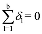. In this case β₀ is given by.

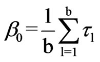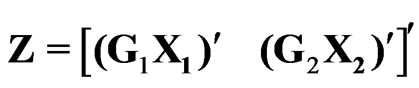
The Equation (4) can be written as

where, , 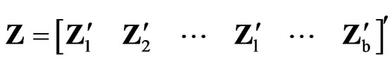Z_l = G_lX_l and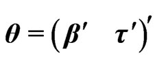. The least square estimate of θ is given by

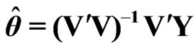
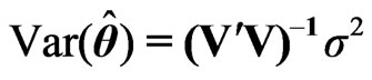
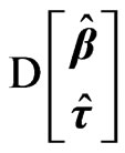
and the variance-covariance of is

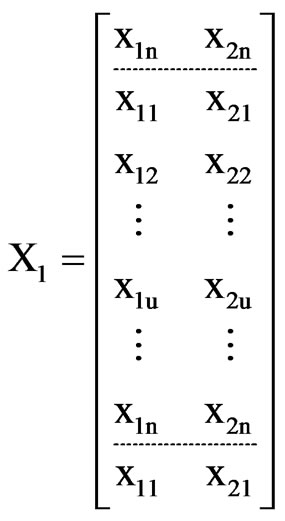
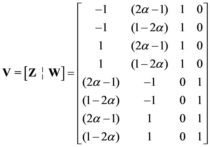
Let v = b = 2 and n₁ = n₂ = n. X_l (l = 1, 2) is of order (n + 2) ´ 2. Hence,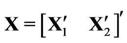. Assuming the same neighbour structure in both the blocks, the n ´ (n + 2) neighbour matrix G_l is as defined in (3).

    Block I          Block II

, ,

. Thus,

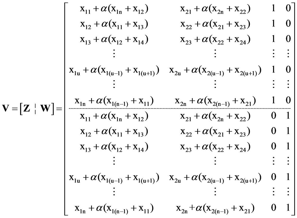
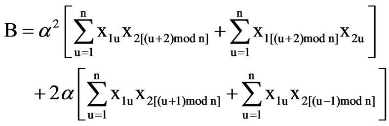
Therefore,

where,

,

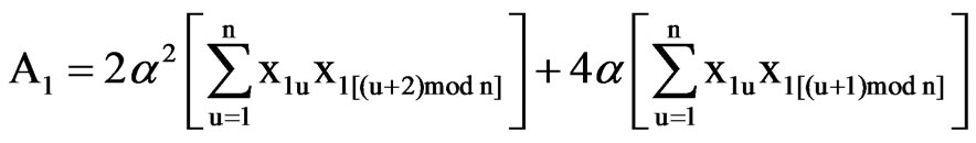and

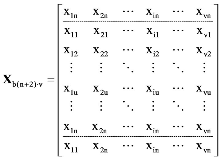
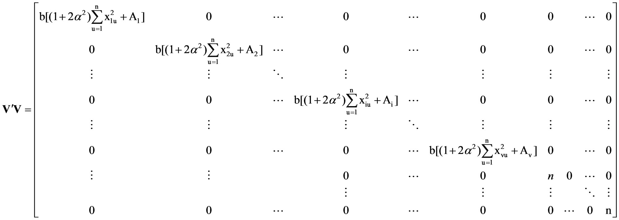
In general for v factors and for b blocks, the X matrix with two extra points as border points is

and so on

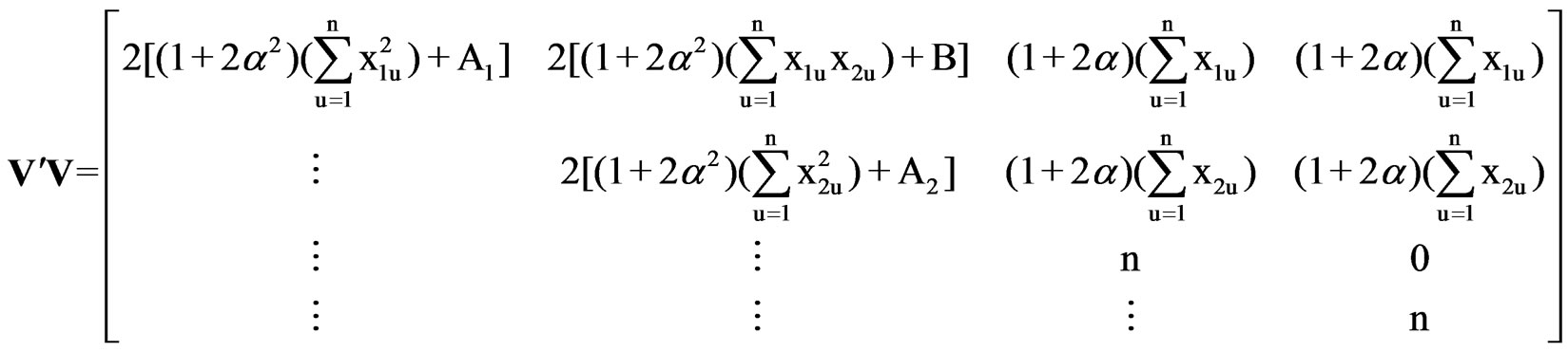
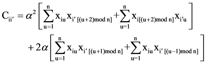
Thus, V´V is obtained as

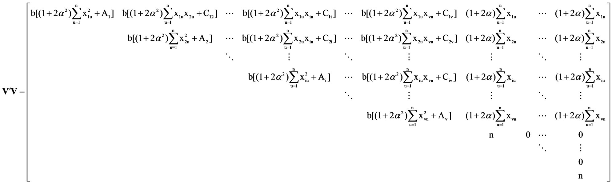
where,

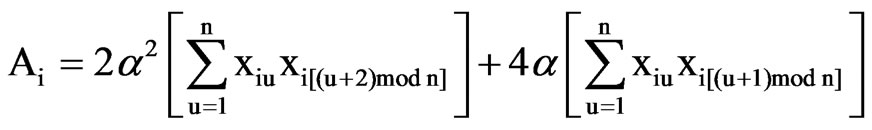
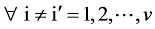
and

.

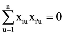
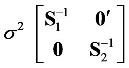
2.2. Conditions for Orthogonality

To ensure orthogonality in the estimation of the parameters, has to be diagonal. This gives rise to the following conditions:

1)

2)

3) 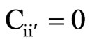for all blocks of size n.

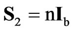
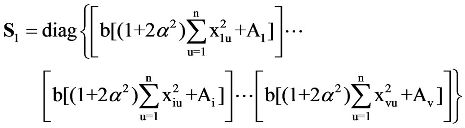
Thus, in view of above conditions, can be written as:

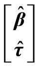
The normal equations for the estimation of (v + b) parameters are

i.e., 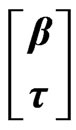= (5)

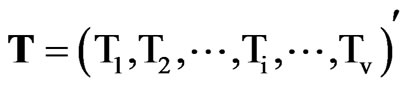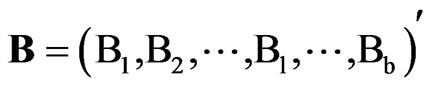where and are the parameters to be estimated. and are the vector of treatment combination totals and block totals respectively, 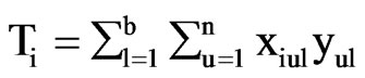and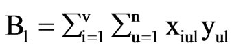, i = 1, 2, …, v and l = 1, 2, ..., b.

Hence,

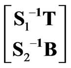= (6)

and

=. (7)

We thus obtain the variance of parameter estimates as

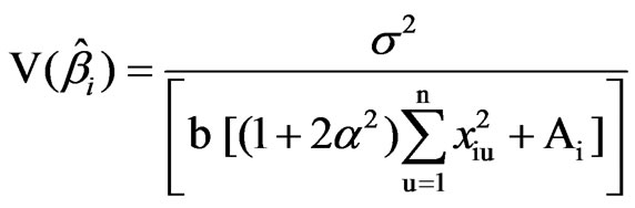and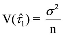for i = 1, 2,…,v, and l = 1, 2, …, b. The estimated response at the point 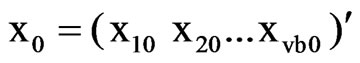is 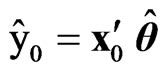with its variance

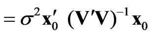
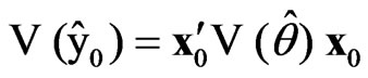
Thus,

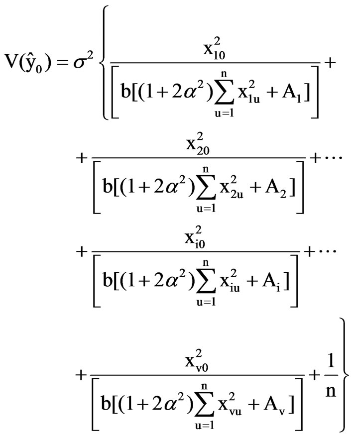(8)

2.3. Conditions for Constancy of the Variances

The constancy of the variances of the parameter estimates is ensured by the following conditions:

1), a constant

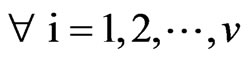
2) A_i = A, a constant for all blocks of size n.

Therefore,

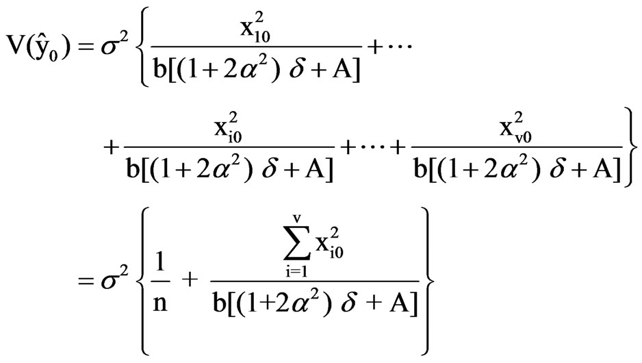(9)

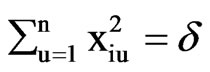
It is thus seen that the variances of b_i’s (i = 1, 2,…, v) are same and the variance of the estimated response is a function of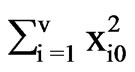. For given, the points for which is same, the estimated response will have the same variance.

3. Method of Construction

Consider a 2^v full factorial for v factors each at 2 levels and arrange the combinations in lexicographic order. Put all these runs in a single block. The second block can be obtained by circularly rotating the columns of first block once. Similarly, rotating the v columns of 2^v factorial points (v – 1) times we get v × 2^v design points in v blocks each of size 2^v. The design so obtained satisfies all the conditions obtained in Section 2. Two extra units are added as border units in each block for neighbour effects.

Illustration

Let v = 2 (X₁ and X₂) with each factor at two levels, then we get four runs in full factorial. The four runs constitute the first block and the other block can be obtained by rotating the columns of the first block in a circular fashion. The various matrices are obtained as follows:

Block I          Block II

;

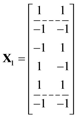
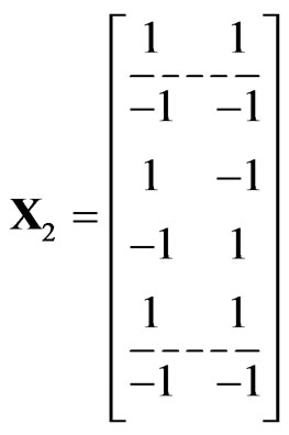
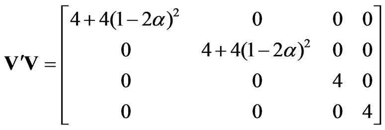
Thus,

for i = 1, 2.

and

for l = 1, 2.

For,

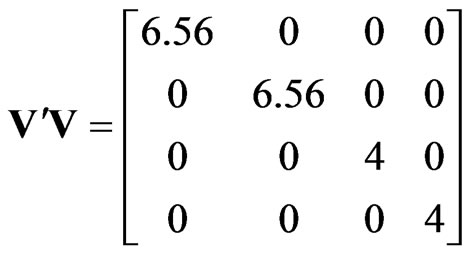
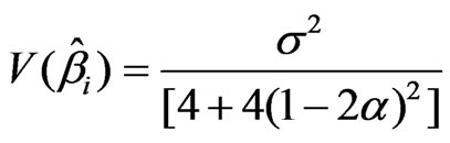
Thus,

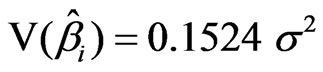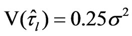, and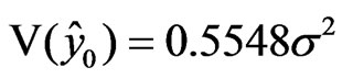

Thus, it is seen that the variance of the estimated response at all points is same.

4. Conclusions

The presence of block effects in a response surface model can affect the estimation of mean response, as well as in determination of the optimum response. Hence, blocking should be done in response surfaces wherever heterogeneity among experimental units is suspected. It has also been shown that incorporating neighbour effect in a model along with block effects results in better estimates of the parameters. The developed methodology and designs can be used to fit the response surfaces with block effects and incorporating neighbour effects.

5. Acknowledgements

We are grateful to the referee and the editor for the valuable suggestions which helped in improving the quality of the paper.

6. References

[1]    A. I. Khuri and J. A. Cornell, “Response Surfaces-Designs and Analysis,” Marcel Dekker, New York, 1996.

[2]    R. H. Myers, D. C. Montgomery and C. M. Anderson, “Response Surface Methodology-Process and Product Optimization using Designed Experiments,” John Wiley Publication, New York, 2009.

[3]    N. R. Draper and I. Guttman, “Incorporating Overlap Effects from Neighbouring Units into Response Surface Models,” Applied Statistics, Vol. 29, No. 2, 1980, pp. 128-134. doi:10.2307/2986297

[4]    Sarika, S. Jaggi and V. K. Sharma, “Second Order Response Surface Model with Neighbour Effects,” Communications Statistics: Theory and Methods, Vol. 38, No. 9, 2009, pp. 1393-1403.

[5]    S. Jaggi, A. Sarika and V. K. Sharma, “Response Surface Analysis Incorporating Neighbour Effects from Adjacent Units,” Indian Journal of Agricultural Sciences, Vol. 80, No. 8, 2010, pp. 719-723.