American Journal of Computational Mathematics
Vol.3 No.2(2013), Article ID:33547,10 pages DOI:10.4236/ajcm.2013.32022
Computational Studies of Reaction-Diffusion Systems by Nonlinear Galerkin Method
Department of Mathematics, Faculty of Nuclear Sciences and Physical Engineering, Czech Technical University in Prague, Prague, Czech Republic
Email: kolarmir@fjfi.cvut.cz
Copyright © 2013 Miroslav Kolář. This is an open access article distributed under the Creative Commons Attribution License, which permits unrestricted use, distribution, and reproduction in any medium, provided the original work is properly cited.
Received April 2, 2013; revised May 1, 2013; accepted May 25, 2013
Keywords: Nonlinear Galerkin Method; Scott-Wang-Showalter Model; Compactness Method
ABSTRACT
This article deals with the computational study of the nonlinear Galerkin method, which is the extension of commonly known Faedo-Galerkin method. The weak formulation of the method is derived and applied to the particular ScottWang-Showalter reaction-diffusion model concerning the problem of combustion of hydrocarbon gases. The proof of convergence of the method based on the method of compactness is introduced. Presented results of numerical simulations are composed of the computational study, where the nonlinear Galerkin method and Faedo-Galerkin method are compared for the problem with analytical solution and the numerical results of the Scott-Wang-Showalter model in 1D.
1. Introduction
It is well known that many problems often occur when one tries to approximate the complex dynamics of reaction-diffusion equations. Especially the error estimate of common methods grows exponentially in time. One possible approach to overcome this problem, known as the Nonlinear Galerkin method is suggested by Marion and Temam in [1]. It is also discussed in [2] and [3]. In this paper we discuss this method and its properties, and apply it to the solution of particular reaction-diffusion model and perform a computational study when the method is compared with the commonly known Faedo-Galerkin method.
Consider a system of reaction-diffusion equations
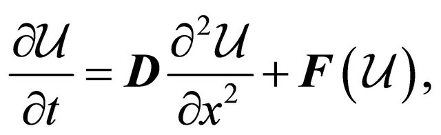 (1)
(1)
where  denotes a positive definite diagonal matrix,
  is a Lipschitz continuous map and
  is a d-dimensional function of time
  and space
 . We consider the homogeneous Dirichlet boundary conditions
  and the initial conditions
 (2)
(2)
We introduce the space 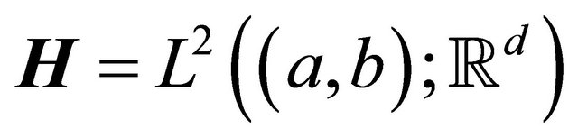 as the Hilbert space with the scalar product
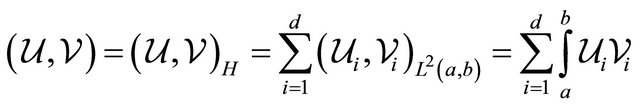 (3)
(3)
and the space 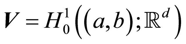 as a Hilbert space endowed with the scalar product
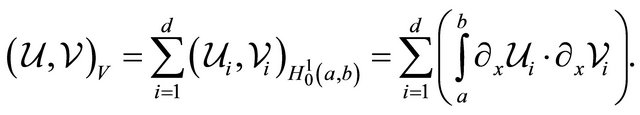 (4)
(4)
Let . Then the weak solution of the problem (1)-(2) on time interval
  is a mapping
  such that it satisfies the following equations for each
 :
:
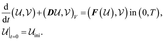 (5)
(5)
2. Nonlinear Galerkin Method
The nonlinear Galerkin method proposed by Marion and Temam in [1] is an extension of the classical FaedoGalerkin method, which is extensively discussed in [4], [2] or [3]. Generally there are two main goals we would like to achieve by using the nonlinear Galerkin method:
• To increase the accuracy of the approximation regarding the computational time of the Faedo-Galerkin method;
• To decrease computational time regarding to the precision of the approximation of the Faedo-Galerkin method.
Analogically to the Faedo-Galerkin method, we search the approximate solution on some finite-dimensional subspace of . Consider a differential equation for the unknown function
  in the following form:
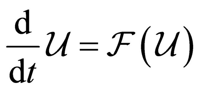 (6)
(6)
with the initial condition
where the mapping  is written as
 for some linear operator
 . The
. The  is a separable Hilbert space with the orthonormal basis
  composed of eigenvectors of the operator
  satisfying the homogeneous Dirichlet boundary conditition in
 .
.
Then we denote symbols  and
and  as projectors to the subspaces
  and
and
 , respectively. Thus
  is a finite-dimensional subspace of
  generated by first m basis functions and
  is its orthogonal complement.
Then, the solution  of Equation (6) can be written as
 (7)
(7)
where
Substituting the decomposition (7) to (6) and applying the operators  and
and , we get
 (8)
(8)
 (9)
(9)
Discretization in the nonlinear Galerkin method is based on the two following steps:
1) Replacing the right hand side  by the first order Taylor expansion:
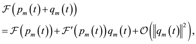
where  is the Jacobian matrix of
 . One suggested approach is that the remainder in the Taylor expansion satisfies these following properties (see [1,2,5]):
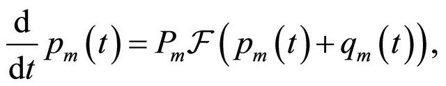
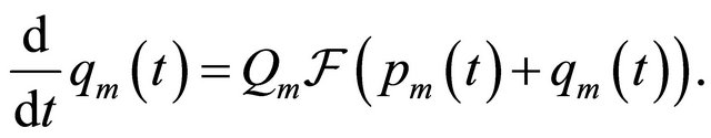
This simplification is implied by a particular nonlinear Galerkin method we are using. Then, the second equation of the system (8) can be written as
2) Replacing the  by some finite-dimensional subspace, since we can only operate on some finitedimensional subspace
  for
for  instead of the whole
  during the numerical computation. Then the
  is replaced by
  and instead of function
 , we consider the function
The equations for the nonlinear Galerkin method can be finally written as the following:
 (10)
(10)
The degree of approximation is determined by the parameters m and M. We interpret the function  as an approximation of solution of (6) in the space
  and
and  as a correction term which modifies
  for large values of time t.
The weak formulation of (10) is obtained easily by multiplicating (10) by basis function  for
for  . Utilizing the orthogonal projection and orthonormality of basis functions
 , we obtain the weak formulation of the nonlinear Galerkin method
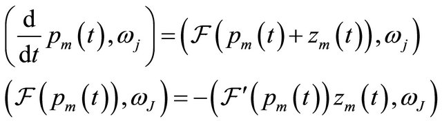 (11)
(11)
for the indices  and
and . We endow these equations with the initial conditions
3. Application to the Scott-Wang-Showalter Model
We show the application of the nonlinear Galerkin method on the particular reaction-diffusion system. It was experimentally discovered, that there arise patterns created by flames during the combustion of mixed compounds of hydrocarbon gases.
This phenomenon is described by the Sal’nikov model (see [4,6,7]), which generates the thermokinetic oscillations. The Sal’nikov’s work deals with the problem of the cool flames during the oxidation of hydrocarbon gases.
The scheme of the Sal’nikov’s thermokinetic oscillation is the following:
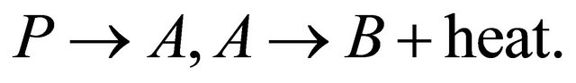
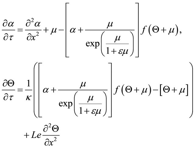
In the first reaction, the compound P generates the reactive compound A. In the second reaction, the compound A decomposes to the inert product B during the emergence of heat. The detailed physical point of view is discussed in [6]. The system of reaction-diffusion equations for dimensionless concentration  of reaction intermediate A and dimensionless temperature
  of reaction compounds is:
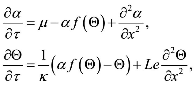 (12)
(12)
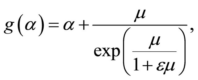
where the function f is defined as
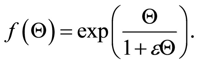 (13)
(13)
The  and the
  are the parameters of the model,
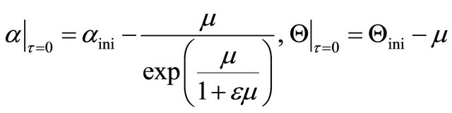
  is the dimensionless time. We complement these equation with the initial conditions
 (14)
(14)
and with the Dirichlet boundary conditions
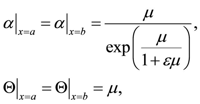 (15)
(15)
which are the stationary solutions of the (12). We convert the problem (12)-(14) into the homogeneous boundary conditions problem. By subtracting the boundary conditions (15) from  and
and  we obtain the system
 (16)
(16)
endowed with the homogeneous boundary conditions and with the following initial conditions
 (17)
(17)
We consider the unknown functions  and
and  as mappings from the interval
  to the
 . Denoting
we introduce the following operator notation for unknown vector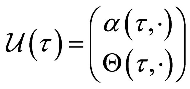 :
:
where
 .
.
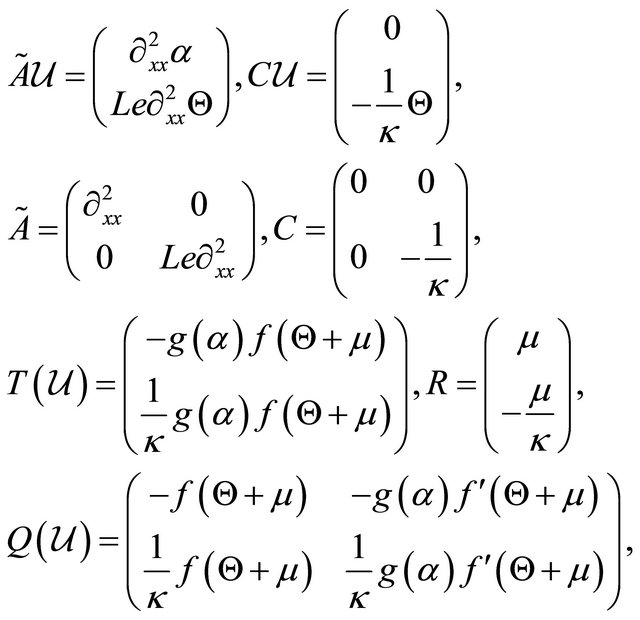
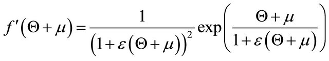
Then we define the operator F as
 with the Jacobian matrix
 . Utilizing this notation, we can rewrite the problem (16)-(17) as
 (18)
(18)
 (19)
(19)
In this case, we consider , the domain
  and the spaces
  and
and
 . Let us denote
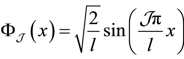 . For the application of the nonlinear Galerkin method, we use the orthonormal basis of
  composed of eigenvectors of the operator
 :
:
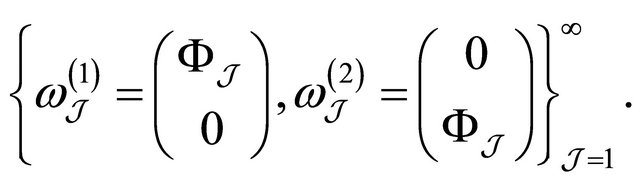 (20)
(20)
We search the Galerkin approximation of  as the decomposition
 , where the approximation term
  and the correction term
  are written as
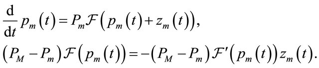
The unknown combination coefficients  and
and  for the
  are given by the following system of differential-algebraic equations:
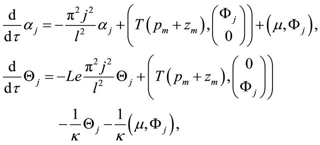 (21)
(21)
for ,
,
 (22)
(22)
for .
.
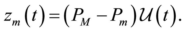
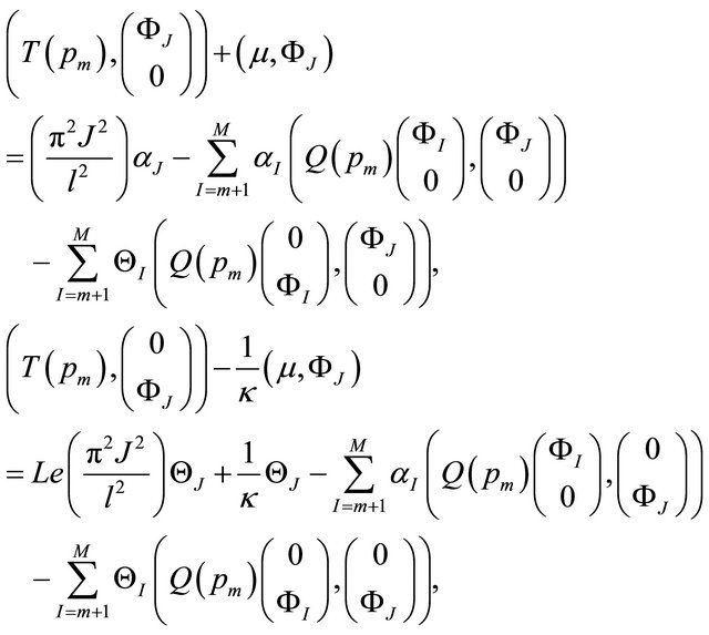
Multiplicating the second equation of (22) by , using simple algebraic manipulations and subtracting it from the first equation of (22), we obtain a linear relation between
  and
and :
:
 (23)
(23)
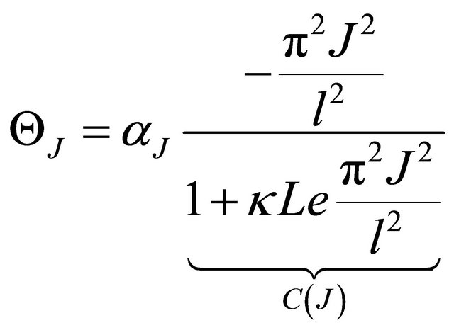
for . The system (22) for correction (with dimension
 ) can be reduced to a system with the dimension equal to
  for the unknown coefficients
 :
:
The coefficients  are then computed via the relation (23).
4. Convergence
We prove the convergence of the nonlinear Galerkin method applied to the Scott-Wang-Showalter model.
The most important note is the existence of the invariant region for the Scott-Wang-Showalter model. Its existence was proved in [7].
We introduce the following operator notation
where Id is the identical operator. The Jacobian matrix of the operator G is computed as
 . Considering the invariant region for the model, the operator G satisfies the Lipschitz condition with the constant
  for each
  and each solution with the initial condition inside te invariant region is bounded, i.e.
 ,
,  for some
  and for each
  and each
 . Then we have the following estimates for the right hand sides of the model
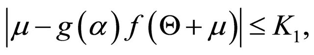
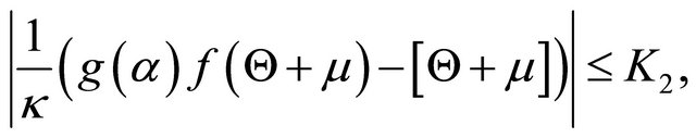
where . Hence we can write the following important estimates for the operator
 :
:
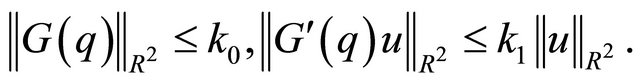 (24)
(24)
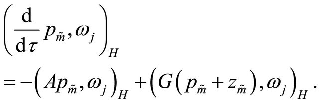
Then the equations for the nonlinear Galerkin method (11) are as follows
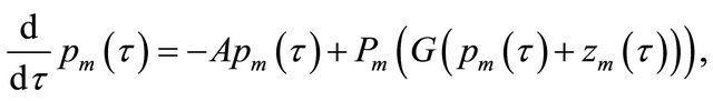
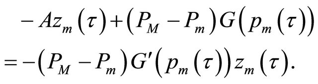 (25)
(25)
Problem (25) is the system of differential-algebraic equations solvable on  due to the theory of ODEs as the algebraic system for
  is uniquely solvable and smoothly depends on
 . The value of
  depends on the quality of approximation.
1) Operator A
The operator  has the same eigenfunctions as the operator
 :
:
The eigenvalues are1 ,
,
 . The operator
  is (see [8]) positive and self-adjoint. Hence we can define its square root
  as
as  for each
 .
.
Now we introduce some useful relations between the operator norms which we use in the next part. For more detailed derivation see [4]
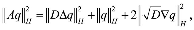 (26)
(26)
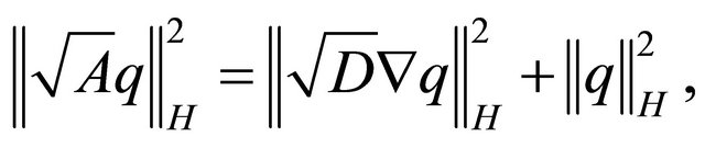 (27)
(27)
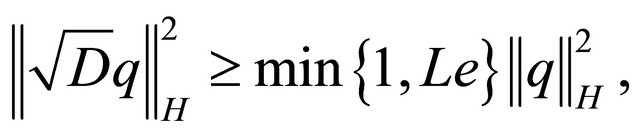 (28)
(28)
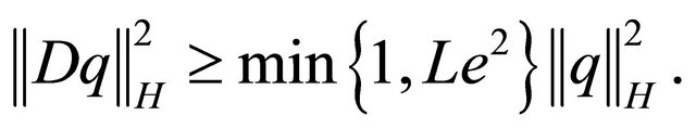 (29)
(29)
To prove the convergence of the nonlinear Galerkin method we process the particular sequences in Equation (25).
2) Sequence 
We multiply the second equation of (25) scalarly by 
Using the Young inequality, we obtain
According to [1], the expression  has its lower bound
and then we can write
Using estimates (24), we obtain
We use relations (27) and (28) on the left hand side of this inequality. Then we obtain the estimate for  via the Poincaré inequality:
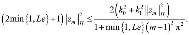
Hence  for
for  uniformly on the interval
 .
.
3) Sequence 
 a
a  are linear operators. We suppose that initial condition
 . Using the Bessel inequality, we obtain following auxiliary estimates
 (30)
(30)
We multiply the first equation of (25) scalarly by 
Using the definition of the square root of operator A, we obtain
We use the Young inequality and (24) to estimate the left hand side and then we obtain the auxiliary estimate
 (31)
(31)
4) Boundedness of  in
in 
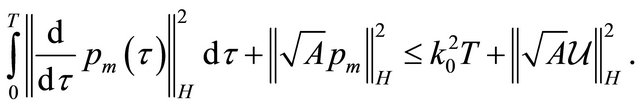
We integrate the Equation (31) over :
:

Dropping the  and using(30) we obtain
Hence the sequence  is bounded in
  for each
 .
.
5) Boundedness of  in
in 
We integrate the Equation (31) over :
:
Dropping the integral of nonnegative function and using (30) we obtain
Hence the sequence  is bounded in
 for each
 .
.
6) Boundedness of 
Using the relations (26) and (27) we get the inequality
The auxiliary relation (31) then leads to
Using the Grönwall lemma for ,
,  and
and  we obtain
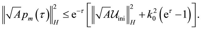
Hence the sequence  is bounded in
  .
.
7) Sequence 
We multiply the first equation of (25) scalarly by :
:
We use the Young inequality for  on the last term and estimate the middle term.
Using the boundedness of the operator G (24) we obtain
We integrate this inequality over  and use the relations (30):
Hence the sequence  is bounded in
 .
.
9) Passage to the limit
Considering the previous estimates (boundedness of  and (27) particularly), we obtain the following properties

whereas
Hence the sequence  is bounded in
  for each
 . This means that we can choose a subsequence
 , which converges weakly in
 .
.
Using the Aubin Lemma (see [9]) for following function spaces:
we obtain that the Banach space
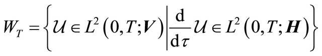
with norm
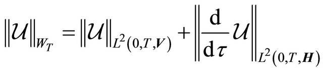
is compactly embedded in .
.
Since the sequence  is bounded in
 and sequence
  is bounded in
  for each
 , there exists a subsequence
 , which converges strongly to the limit point p in
 . Knowing that the sequence
  converges weakly in
 , we obtain from uniqueness of the limit that
 .
.
10) Sequence 
Since the operator  satisfies the Lipschitz condition, we can perform the following estimate
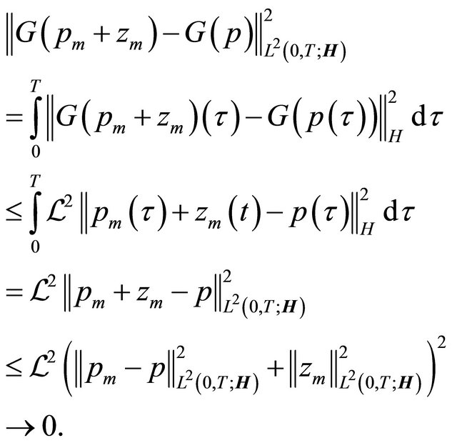
Hence  strongly in
 .
.
11) Existence and uniqueness of weak solution
In this part we prove the existence and uniqueness of the weak solution of the Scott-Wang-Showalter model. The existence is proven via the strong convergence of the sequence .
.
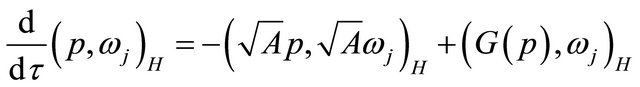
We multiply the first equation of (25) by  for
for .
.
Multiplying the previous relation by the test function ,
,  and integrating it over
  we obtain
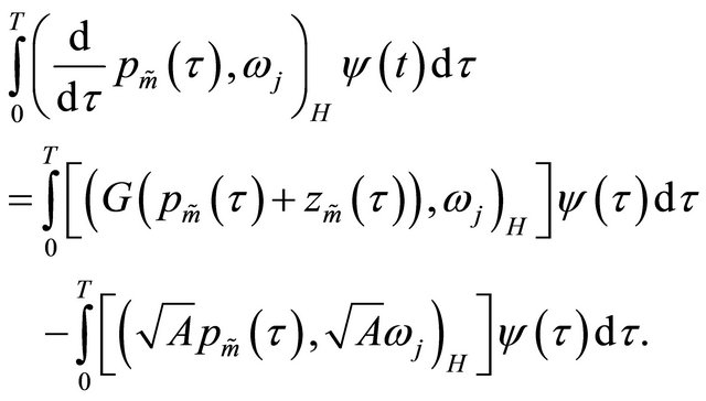
Integrating the left hand side per parts and passing to the limit we obtain
 (32)
(32)
Additionally, we consider . Then
 (33)
(33)
in sense of distributions.
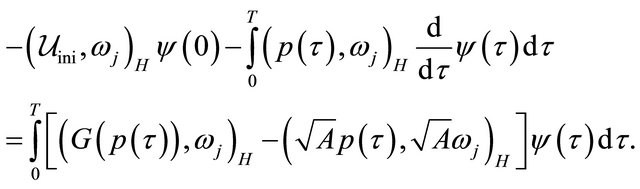
Now, we multiply the Equation (33) by ,
,  and integrate it over
 . Using integration per parts we obtain
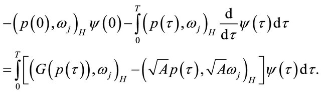 (34)
(34)
Subtracting (32) and (34) we get
which means that . Hence
  is the weak solution.
To show the uniqueness, we suppose there are two different weak solutions  and
and , which satisfy
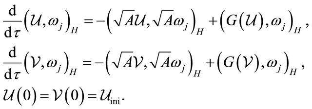
We denote . Then we subtract the previous equations, multiply it by
  and sum it over
 .
.
Hence
Finally, using the Young inequality for the last term and Lipschitz condition of operator , we obtain
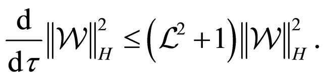
Choosing  and
and , we use the Grönwall lemma:
Hence  for each
 , which is the contradiction.
5. Quantitative Analysis
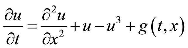
In this paper we deal with the error measurement and computational time of the nonlinear Galerkin method aplied to a particular reaction-diffusion model. We are interested in the long-term behaviour in particular. It is clear that the accuracy and computational time of the nonlinear Galerkin method depends on the dimension of the function subspace, where the approximation of the solutions is searched. Before the application on the ScottWang-Showalter model, we use the single one-dimensional reaction-diffusion equation with the known analytical solution  as a benchmark for the method. Consider the equation
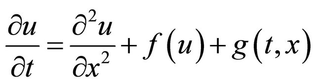 (35)
(35)
for  and
and  satisfying the homogeneous Dirichlet boundary condition and initial condition
 (36)
(36)
where f is a nonlinear function of u and g is a chosen function of time  and space
 , such that u is the analytical solution of the problem (35)-(36). In all simulations we use either
 ,
,  (which is the case of the commonly known Faedo-Galerkin methodsee [4]) or
 ,
,  in the Galerkin approximation.
The explicit form of function  for all discussed cases, equations for the nonlinear Galerkin approximation and enumerated scalar products can be easily derived or found in [4].
The systems of ordinary differential equations for approximation from the nonlinear Galerkin method are solved by means of time-adaptive Runge-Kutta-Merson method. The linear systems for correction are solved via Gauss elimination method since they are generally a systems with dense matrices.
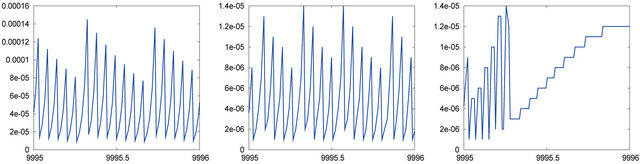
We plot the  norm of the difference between analytical solution and numerical approximation, i.e.
  in specific time intervals. Time is measured in seconds. Additionally, Table 1 of computational complexity is included.
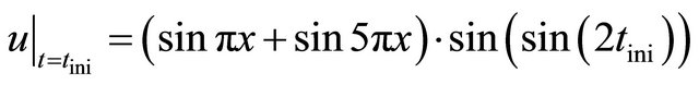
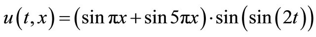
5.1. Simulation 1
Consider equation
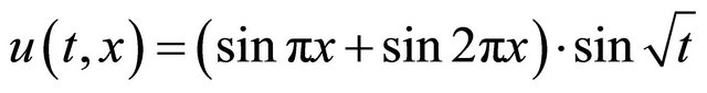
with initial condition  and with the analytical solution u in form
 . The time evolution of error is on the Figures 1 and 2.
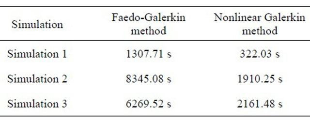
Table 1. Computational complexities for testing simulations.
 (a) (b) (c)
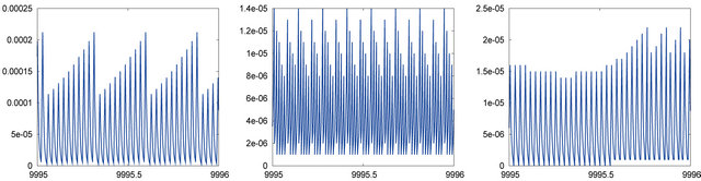
Figure 1. Time evolution of errors for the Faedo-Galerkin method. (a) Simulation 1; (b) Simulation 2; (c) Simulation 3.
 (a) (b) (c)
Figure 2. Time evolution of errors for the nonlinear Galerkin method. (a) Simulation 1; (b) Simulation 2; (c) Simulation 3.
5.2. Simulation 2
Consider equation
with initial condition 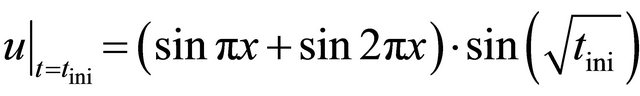 and with analytical solution equals to
 . The time evolution of error is on the Figures 1 and 2.
5.3. Simulation 3
Consider equation

with initial condition
and with analytical solution equals to
 .
.
The time evolution of error is on the Figures 1 and 2.
6. Qualitative Studies
In this section we present the computational results for the Scott-Wang-Showalter model. Considering the homogeneous boundary condition problem (16)-(17), we investigate the behaviour of the model depending on various initial conditions and various sets of parameters. Additionally, deeper computational study can be found in [4]. The following figures show the time evolution of function .
.
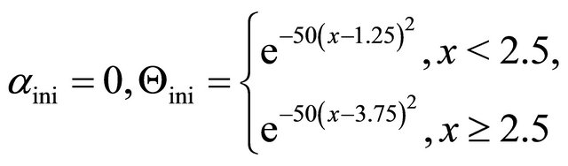
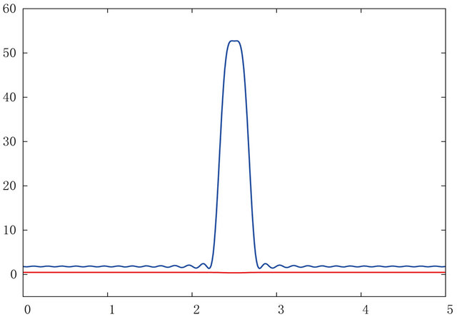
6.1. Simulation 4
We solve the homogeneous boundary condition problem (16)-(17) with the following initial conditions
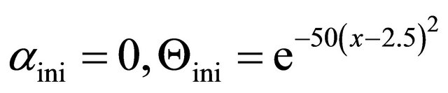 (37)
(37)
for . The parameters of the model are
  and the number of modes in the Galerkin approximation is
 . The time evolution of the problem is on the Figure 3.
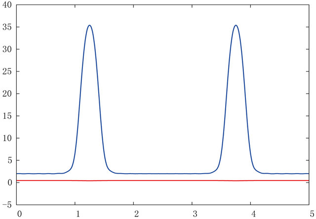
6.2. Simulation 5
We solve the homogeneous boundary condition problem (16)-(17) with the following initial conditions
 (38)
(38)
for . The parameters of the model are
 (a)
(a)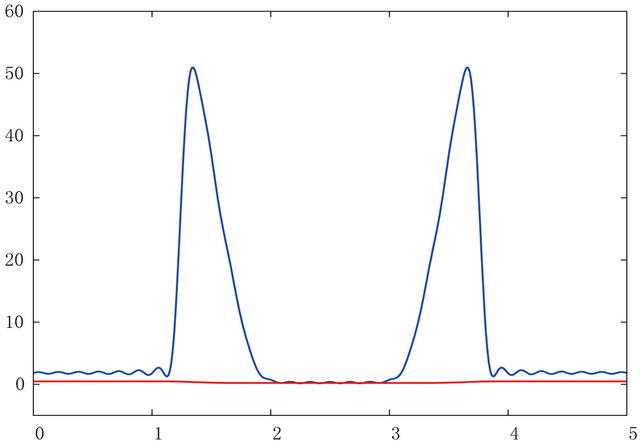 (b)
(b)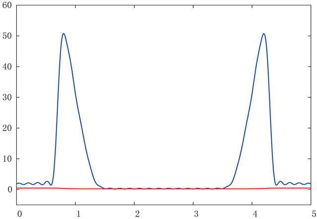 (c)
(c)
Figure 3. Simulation 4—time evolution of the functions Θ (blue line) and α (red line). (a) τ = 0.00614; (b) τ = 0.01814; (c) τ = 0.02214.
 and the number of modes in the Galerkin approximation is
 . The time evolution of the problem is on the Figure 4.
7. Conclusion
In this paper we applied nonlinear Galerkin method to
 (a)
(a)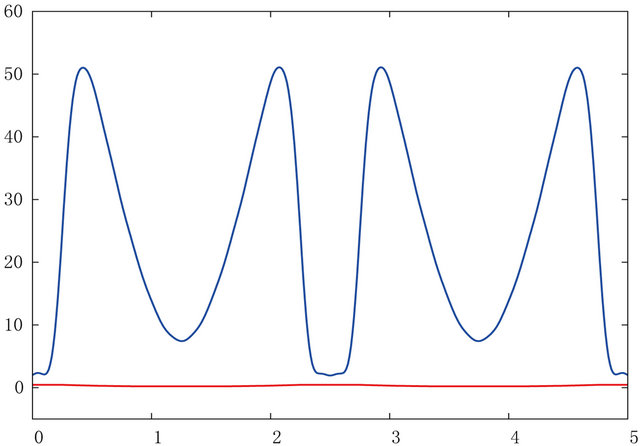 (b)
(b)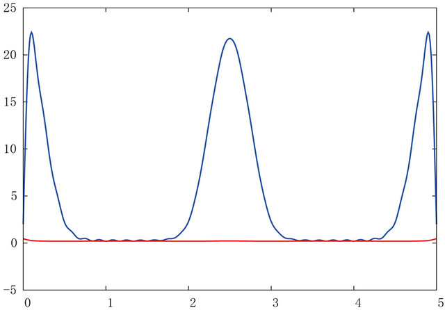 (c)
(c)
Figure 4. Simulation 5—time evolution of the functions Θ (blue line) and α (red line). (a) τ = 0.00511; (b) τ = 0.01311; (c) τ = 0.02025.
the particular system of reaction-diffusion equations in one spatial dimension. As the investigated reaction-diffusion system was chosen the Scott-Wang-Showalter model. We presented the system of differential-algebraic equations for the approximation of the weak solution, proof of existence and uniqueness of the weak solution and the proof of convergence of the nonlinear Galerkin method. We performed quantitative analysis among analytical solution and numerical approximations obtained via the nonlinear Galerkin method and the commonly known Faedo-Galerkin method. It indicates that the nonlinear Galerkin method is more efficient since it conserves the similar level of accuracy with respect to the shorter computational time.
8. Acknowledgements
Partial support of the project No. TA0102871 of the Technological Agency of the Czech Republic, No. SGS11/161/OHK4/3T/14 of the Czech Technical University in Prague, No. MSM 6840770010 of the Ministry of Education, Youth and Sport of the Czech Republic is acknowledged.
REFERENCES
- M. Marion and R. Temam, “Nonlinear Galerkin Methods,” SIAM Journal on Numerical Analysis, Vol. 26, No. 5, 1989, pp. 1139-1157. doi:10.1137/0726063
- J. Šembera and M. Beneš, “Nonlinear Galerkin Method for Reaction-Diffusion Systems Admitting Invariant Regions,” Journal of Computational and Applied Mathematics, Vol. 136, No. 1-2, 2001, pp. 163-176. doi:10.1016/S0377-0427(00)00582-3
- J. Mach, “Application of the Nonlinear Galerkin FEM Method to the Solution of the Reaction Diffusion Equations,” Journal of Math-for-Industry, Vol. 3, 2011, pp. 41-51.
- M. Kolář, “Mathematical Modelling and Numerical Simulations of Reaction-Diffusion Processes,” Diploma Thesis, Department of Mathematics FNSPE CTU, Prague, 2012.
- A. Debussche and M. Marion, “On the Construction of Families of Approximate Inertial Manifolds,” Journal of Differential Equations, Vol. 100, No. 1, 1992, pp. 173- 201. doi:10.1016/0022-0396(92)90131-6
- S. K. Scott, J. Wang and K. Showalter, “Modelling Studies of Spiral Waves and Target Patterns in Premixed Flames,” Journal of the Chemical Society, Faraday Transactions, Vol. 93, No. 9, 1997, pp. 1733-1739. doi:10.1039/a608474e
- V. Tomica, “Reaction-Diffusion Equations in Combustion,” Proceedings of Czech Japanese Seminar in Applied Mathematics, Prague, 30 August-4 September 2010, pp. 84-93.
- R. Temam, “Infinite-Dimensional Dynamical Systems in Mechanics and Physics,” Springer, Berlin, 1997.
- J. L. Lions, “Quelques Méthodes de Résolution des Problémes aux Limites non Linéaires,” Dunod, Paris, 1969.
NOTES
1Denoting the  the largest one and the
  the smallest one.