Received 6 January 2016; accepted 7 March 2016; published 10 March 2016

ABSTRACT

This paper studies firms’ innovation behavior in a supply chain where two firms first invest to reduce component’ cost according to different innovation modes (non-cooperative innovation, sequential innovation, and cooperative innovation) and then decide the prices according to different market powers (Supplier-Stackelberg, Manufacturer-Stackelberg, and Nash). We find that both the supplier and the manufacturer make more innovation efforts and profits under sequential innovation than under non-cooperative innovation when the market power is any one of three structures. Moreover, the firm prefers to invest as the follower in sequential innovation. We also show that the firms are easy to achieve cooperative innovation under symmetrical power market structure than asymmetrical power market structure. By using a concept named innovation-desirability- index that measures a firm’s desire to innovate in the supply chain, we show that it is optimal for a firm in the chain to cooperate with such a firm whose market power is close to his own if the innovation-desirability-index is higher, otherwise with such a firm whose market power is lower to his own.

Keywords:

Supply Chain, Innovation Mode, Market Power, Game Theory

1. Introduction

Businesses are increasingly relying on their suppliers to reduce costs, improve quality, and develop new processes and products faster than their rivals’ vendors can. In some industries, the method of helping suppliers to reduce components’ cost has been applied very successfully, for example, Toyota and Honda. Toyota’s Construction of Cost Competitiveness for the 21st Century (CCC21) program, which aims at 30% reduction in the prices of 170 parts that the company buys for its next generation of vehicles. The supplier didn’t decry CCC21 as unfair. Instead, Toyota would help them achieve that target by making their manufacturing processes leaner, and because of Toyota’s tough love, they would become more competitive and more profitable in the future [1] . In general, cost reduction investments involve long lead times and often need to be committed before the end product is revealed. Therefore, in our setting, such investments are committed on the first stage, which is called innovation stage. Due to spillover effect, investment in innovation by each firm will benefit both supply chain partners. How they decide their investment levels? There are several modes. The supplier and the manufacturer can form a cartel to coordinate their investment decisions, called Cooperative Innovation (denoted as mode C). The supplier and the manufacturer make investment decisions simultaneously and independently, called Non-cooperative Innovation (denoted as mode N). Moreover, the timing of investment decisions can influence the investment decisions due to fear of opportunism. For example, recently, Intel announced to invest $10 billions in US to build the laboratory to help original equipment manufacturers (OEMs), who develop electronic commerce platform in the architecture of the Intel Server, then a large number of OEMs take part and invest. So Sequential Innovation means that the supplier (or the manufacturer) is the first mover to invest, and then the manufacturer (or the supplier) decides its investment (denoted as mode S or M).

On the other hand, pricing decisions, i.e., the supplier’s wholesale pricing and the manufacture’s resale pricing, can be postponed until after the cost reduction is observed. Therefore, such pricing decisions are decided on the second stage, called the price competition stage. If the supplier possesses more bargaining power than the manufacturer, the interactions between supply-chain partners will follow a Supplier Stackelberg model. However, if the manufacturer possesses more negotiation power due to its dominating size or customer loyalty, the supply chain follows the Manufacture Stackelberg model. If neither the manufacturer nor the supplier possesses a larger bargaining power in negotiations, the supply chain interaction then follows a Nash model. This article develops the models considering all three scenarios. A number of studies have been reported with regard to various power structures in a supply chain (e.g., [2] -[4] .). However, to the best of our knowledge, no research has considered the cooperative innovation problem in a supply chain by considering the firms’ market powers. The detailed definitions for the innovation modes and market powers are given in Section 2. Then several questions naturally arise as follows: 1) How do firms choose different innovation modes? 2) Does an optimal innovation mode exist in terms of profitability? 3) How do the market powers affect the level of innovation they provide to each other? 4) How do the investment and pricing decisions are inter-linked? We seek to address the above questions in this paper.

We consider a supplier (S) who sells a component to an independent manufacturer (M). In the first stage, both firms decide their investments on supplier’s cost reduction according to some specified innovation modes and in the second stage, two firms determine their prices according to different market power structures. We introduce a concept named innovation-desirability-index that depends on firms’ technological parameters and sensitivity of market price related to the final product. Our main findings are as follows. First, in any kind of market power structures, both the supplier and the manufacturer are better off under sequential innovation. In practice, sequential innovation is common. Second, in any kind of innovation modes, it is optimal for a firm to cooperate with such a firm whose market power is close to his own in the chain if the innovation-desirability-index is higher, otherwise with such a firm whose market power is lower to his own. Third, the supply chain makes more total profits, but the profits of the supplier and manufacture do not necessarily increase under cooperative innovation. That is, the supplier and the manufacturer have incentives to form cooperative innovation, if and only if certain conditions are established. Finally, the supplier and the manufacturer are easy to achieve cooperative innovation under symmetrical power market structure than asymmetrical power market structure.

There are several related areas to this paper. The first is collaborative innovation in supply chains which has emerged in the recent evolution of operations management research. As indicated in many reports (e.g., [5] ), such an early-stage collaboration in a supply chain is commonplace in many industries. For the collaborative innovation investment, as shown in the literatures, cost reduction is of the main objective (e.g., [6] -[8] ). In this paper, we also focus on cost reduction, which is motivated by widespread practice of such initiatives (e.g., [9] ). Gupta and Loulou [10] and Gupta [11] study how interactions between firms in a channel affect innovation. Gilbert and Cvsa [12] analyze the effect of strategic commitment to price by a supplier to stimulate downstream innovation in a supply chain. Bernstein and Kök [13] investigate cost reduction in an assembly network. All papers above do not consider collaboration. Bhaskaran and Krishnan [14] touch on collaborative product develop- ment decisions and conceptualize and model the revenue, cost, and effort sharing collaborative arrangements between two firms in a supply chain. Kim and Netessine [15] consider collaborative innovation on cost reduc- tion in a supply chain focused on information asymmetry and procurement contract, but they do not consider powers and timing of collaborative decision. Ishii [16] and Ge and Hu [17] consider mode choice for firms of supply chains investing on cost reduction, however, they focus on collaboration mode with spillover. This paper explores firms’ decision sequence and power.

Our paper is also related to firms’ market powers or timing of decisions in supply chains. It is most commonly assumed that manufacturers are more powerful and are leaders of Stackelberg games in Weng (1995). However, as Messinger and Narasimhan [18] and Raju and Zhang [19] point out, market power in some industries has shifted from manufacturers to retailers. Iyer and Villas-Boas [20] give such examples in industries of grocery, construction, and automobile. Dukes et al. [21] discuss market power of large retailers as Wal-Mart. An interesting question is how decisions are affected by market power in supply chains. For a supply chain with two manufacturers and one retailer, Choi [2] analyzes price competition via three non-cooperative games with different power structures: the manufacturer Stackelberg game, the retailer Stackelberg game, and the Nash game. He shows that all members are better off when no one dominates the others. His work is extended by Lu et al. [22] who consider service factors and focus the importance of service from manufacturers in the interactions between two competing manufacturers and their common retailer based on three market power structures. They conclude that consumers receive higher service level when every channel members possess equal market power (e.g., Vertical Nash). Choi’s [2] work is followed by Trivedi [3] , who considers a supply chain in which there are duopoly manufacturers and duopoly common retailers. Trivedi [3] shows that the benefit of the leadership depends on competition level. Ertek and Griffin [23] investigate effect of market power on the supply chain when either the manufacturer or the retailer has dominant power. Wu et al. [4] explore the effect of retail substitutability on the equilibrium quantities in a supply chain that consists of two retailers and one common supplier among six power structures. Zhang et al. [24] investigate the influences of products’ substitutability and channel position in two dual-exclusive channels. It shows that no power structure is always the best for the entire supply chain, and the Nash game is equilibrium for the members. Wei et al. [25] explore the pricing problems with regard to two complementary products in a supply chain with two manufacturers and one common retailer by considering market power.

About the issues of altering the nature of competition by selecting the timing of moves, Amir and Stepanova [26] consider the issue of first versus second-mover advantage in differentiated product Bertrand duopoly with general demand and asymmetric linear costs. Barcena-Ruiz [27] considers endogenous order of moves in a mixed duopoly in which firms determine their pricing decisions simultaneously or sequentially. Granot and Yin [28] analyze sequential commitment in a decentralized newsvendor model with one manufacturer and one retailer under price-dependent demand. Su and Rao [29] develop a game-theoretic model to study the timing of new product preannouncement and launch under competition. Wei et al. [25] provide detailed reviews for this literature. The works above on the timing of decision are not on collaborative innovation.

Our study is closely related to a recent paper of Gurnani et al. [30] , who consider a supply chain with one manufacturer and one retailer. The manufacturer invests in technology to improve product quality, and the retailer invests in selling effort to develop the market before uncertainty in demand is resolved. However, this study differs from Gurnani et al. [30] in the following aspects. First, in comparison to the demand depending on investment and price in Gurnani et al. [30] , we consider the demand depending only on price. Second, while Gurnani et al. [30] focus on the effect of timing of price commitment decisions on the investment decisions and on the profits for the two firms, we use the timing of investment and price decisions to mean different inno- vation modes and market power structures, and explore the interaction between the innovation modes and market power structures. The objective of this study is to focus on different types of decision-making structures. Thus, we study various sequences used by the firms in making both investment and pricing decisions in the supply chain. We are able to show the preference of the supplier and the manufacturer for certain configurations.

The rest of the paper is organized as follows. In Section 2, we introduce our proposed model and derive their equilibria. In Section 3, we comprise the innovation modes given a market power structure. Section 4, we analyze how the market power affect the manufacturer and supplier’ investment decisions and profits. Section 5 is a concluding section.

2. Model and Equilibria

The supply chain studied here consists of two risk neutral firms: a supplier and a manufacturer who buys components from the supplier. The manufacturer transforms components (or intermediate inputs) produced by the supplier into final products. Without loss of generality, we assume that each final product needs exactly one component. The unit production cost at the supplier and the manufacturer are and, respectively. The manufacturer faces linear demand, where is a positive constant representing the size of the potential market, and b is the price-elasticity index of demand. Our model consists of two stages [17] [31] -[33] . In the first stage, both firms decide their innovation investments according to some specified inno- vation modes to reduce the supplier’s production cost, and in the second stage, the two firms determine their prices (wholesale price at the supplier and the retail price at the manufacturer) according to some specified market power structures. The details are given in the following.

For the first stage (cooperative innovation), we assume the innovation investment is quadratic in the level of

cost reduction. That is, effort has to be paid to achieve a cost reduction for firm i, where is a

technological parameter related to marginal innovation effort. Note that the quadratic form has been assumed very commonly in the literatures (e.g., [17] [31] -[33] ). After both firms' innovation efforts, the supplier’s component cost is reduced from the original to. We consider three different innovation modes for the first stage.

Non-Cooperative Innovation (N) The manufacturer and supplier make their innovation investment decisions simultaneously to maximize their own individual profits. Hence they face a Nash game.

Sequential Innovation (S, M) The supplier (manufacturer) first decides his innovation investment decision and the manufacturer (supplier) then makes investment decision.

Cooperative Innovation (C) Both players jointly decide on their innovation investment strategy to maximize the total system profit.

In the second stage (price competition), we consider a two-stage supply chain with different power structures which appear in practice. In some supply chains, the upstream members (e.g., Microsoft and Intel) play a more dominant role than downstream members; however, in some other supply chains, retailers (e.g., WalMart and Tesco) play a more dominant role than upstream members [23] . In a small or local market, both manufacturer and supplier have equal market powers and thus make their decisions simultaneously. Thus, this paper focuses on the following three power structures in the price competition stage.

Supplier-Stackelberg (S) The supplier has dominant market power and has the freedom to decide on wholesale price w to maximize his net profit. The manufacturer then reacts to the wholesale price w declared by selecting her optimal retail price p to maximize her net profit.

Manufacture-Stackelberg (M) The manufacturer becomes the leader and the supplier is the follower. The supplier chooses his wholesale price w conditional on the manufacturer’s retail price or equivalently, the margin on the final product.

Nash Game (N) The supplier and manufacturer have equal power. So, they make their price decisions (w and p) simultaneously and thus face a Nash game.

Given both members’ innovation investments and wholesale price w and retail price p, the profits of the supplier and the manufacturer are, respectively,

The supply chain profit is

We have four different innovation modes in the first stage and three different power structures in the second stage. Thus, we have total 12 settings and will use (xy) to denote the one with the innovation mode (x) and the power structure (y), for x = N, S, M, C and y = S, M, N. Also, the superscript xy is used to indicate the setting. Essentially there is a Stackelberg game underlying each setting.

we first describe the process of cooperation and competition of the non-cooperative innovation under different power structures. There are three scenarios:

Mode (NS) Both firms independently and simultaneously decide their individual innovation investments to maximize their own profits, then the supplier offers a wholesale price w, and finally the manufacturer decides its retail price p. Thus, the game can be described by

Mode (NM) Both firms’ decisions are similar to Mode NS in the first innovation stage, then the manufacture sets its retail margin m, followed by a response from the supplier who determines a wholesale price w. The game can be written as

Mode (NN) Both firms’ decision is also similar to Mode NS in the first innovation stage, and then decide their prices. That is,

Next, we consider sequential investment game with different market power structures. Then, there are six scenarios:

Mode (SS) Here, first the supplier decides its effort level, then the manufacturer decides its effort level, the supplier offers a wholesale price w, and finally the manufacturer decides its retail price p. This process of cooperation and competition can be described by

Mode (MS) Here, first the manufacturer decides its effort level, then the supplier decides its effort level, the price decisions are similar to Mode SS. The game in the chain can be written as

Similarly, the other games can be written as follows:

Mode (SM)

Mode (MM)

Mode (SN)

Mode (MN)

Finally, we consider cooperative innovation with different market power structures. There are three scenarios:

Mode (CS) Both firms jointly decide their innovation investments to maximize the chain profit, then the supplier offers a wholesale price w, and finally the manufacturer decides its retail price p as a response. The game can be described by

Similarly, the other games can be written as follows:

Mode (CM)

Mode (CN)

We solve the games by backward induction. Closed-form equilibrium expressions for investments, prices, demands, and profits are listed in Tables 1-5 (given in the appendix). For simplified expression, we denote, and define. decreases with its own technological parameter, but increases with the sensitivity of market price b. In some sense, indicates the firm i’s desire to innovate. Therefore, for a supply chain member, a small value of represents relatively little desire to innovate, while a large value of represents a relatively greater desire to innovate. So we call the innovation- desirability-index. To ensure the existence and uniqueness of quality-level equilibria under all the modes, it is assumed throughout the paper that, which is proved in the Appendix 6.3. Condition implies that each firm’s desire level should not be too large.

3. Innovation Modes Comparison

We must also understand which innovation mode is better given a market power structure. The following propositions answer this question.

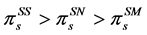
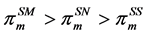
Proposition 1. Given a market power structure, we have,

, and,.

Proposition 1 tells us that both firms invest more in innovation and are better off under sequential innovation than under non-cooperative innovation, given any market power structure. At least one firm should do everything he can to invest, the other firm can promote the increase of the profit through the complementary investment decisions of the firm under sequential innovation. But no early investment commitment leads to the firms all having the risk of over investing under non-cooperative innovation. Therefore, the firms would invest less in innovation, that is,. That leads to lower demand potential for the product, and lower profits for the integrated channel. In practice, sequential innovation is common, such as Toyota’s Opera- tions Management Consulting Division (OMCD) in Japan and the Toyota Supplier Support Center (TSSC) in the US. Dyer and Nobeoka state “The purpose of OMCD is to maintain a group of internal consultants with high levels of expertise in operations to assist in solving operational problems both at Toyota and at Toyota’s suppliers”. Many suppliers have received free assistance in building up lean manufacturing capabilities. These organizational capabilities benefited both suppliers and Toyota in the long run. Then, more and more suppliers are willing to join and innovate with Toyota [34] [35] .

Proposition 2. and, where and.

Proposition 2 tells us that both firms invest the highest one in innovation under the cooperative innovation, followed by the sequential innovation, and the least under the non-cooperative innovation, given any market power structure. Proposition 2 also tells us that the supply chain profits have the same property as the innovation investment. The supply chain profit increases if cooperative innovation is implemented by the two firms, since the objective of cooperative innovation mode is to maximize the total profit while the two firms are competitive in non-cooperative innovation mode and sequential innovation mode in the first stage.

The next proposition compares profits of the members, respectively.

In the next proposition, we let, , and

Proposition 3. 1) and if and only if and or and.

2) and if and only if and or and.

3) and if and only if and or and.

From Proposition 2, the supply chain obtains the highest profit under the cooperative innovation, but this is not necessarily true for the supplier and manufacturer from Proposition 3 except under certain conditions. That is, the supplier and the manufacturer have incentives to coordinate in innovation if and only if certain conditions are established. Proposition 1 tells us that both the supplier and the manufacturer are better off under sequential innovation than under non-cooperative innovation.

Further from Proposition 3, when the market power is asymmetrical, the firm with strong power has incentives to form the cooperative innovation if and only if or; the firm with weak power has incentives to form the cooperative innovation if and only if or. This shows that the condition for the supply chain members reaching a cooperative innovation is of serious difference, that is to say, a cooperative innovation is difficult. When the market power is symmetrical for the two firms, they have incentives to form the cooperative innovation if and only if or. This shows that the condition of the supply chain members reaching a cooperative innovation is of little difference, that is to say, a cooperative innovation is easy. In summary, Proposition 3 tells us that the supplier and the manufacturer are easy to achieve the cooperative innovation under the symmetrical power market structure than under the asymmetrical power market structure.

Overall, The manufacturer and supplier prefer sequential innovation to non-cooperative innovation, but prefer cooperative innovation if and only if certain conditions are established. And the supplier and the manufacturer are easy to achieve the cooperative innovation when market power is symmetrical.

Next, we compare the different sequential innovation modes given the market power. Based on the results summarized in Table 2 and Table 3, we can get the following results.

Proposition 4. 1) and, but and; and.

2), , but and;,.

Suppose the supplier has more market power in the second price competition stage. Proposition 4 tells us that each firm invests more in innovation but earns less as the leader than as the follower in the sequential innovation stage. In mode (SS), the supplier makes the investment in innovation and the wholesale price. Thus, the supplier doesn’t have risk of over investing in innovation. Therefore, the supplier would invest more in innovation, that is,. The manufacturer, in mode (SS) and (MS), makes the investment in innovation before the wholesale price is set. Thus, the manufacturer has the risk of over investing in innovation and faces a high wholesale price from the supplier. The manufacturer is willing to invest more () in mode (MS) because first making the investment in innovation in mode MS can make more demand. Why does each firm

invest more in innovation but earn less? For the supplier, , and, that is, the innovation decisions of the supplier and manufacturer complementary work

together to the supplier profit in mode (MS). But the only innovation decision of the supplier increases the

supplier profit in mode (SS) (, and).

Proposition 4 also shows that more demand and higher chain profit are created when the manufacturer is the leader than the supplier is the leader in the first sequential innovation stage. In mode (MS), the supplier can promote the profit by using complementary decision of the manufacturer in the first stage and allot more profits by using the first-move advantage. In this way, the firm has all the advantages, and it will do its best to achieve profits and make more total profits.

In summary, although the firm as the leader invests more in innovation, both firms are more willing to be the follower in the first stage, while the supply chain creates higher profits when the decision sequence is reverse in the first stage to that in the second stage.

Then, we study how the decision sequence in the first stage affects the firms’ innovation investment levels and profits under the symmetric power structure in the second price compete stage. From Table 4, we have the following result.

Proposition 5. and, but and;,.

Provided the symmetric power structure in the price competition stage, Proposition 5 tells us that the firm, who is the leader, invests more but earns less as the leader than as the follower in the first cooperative innovation stage. This is similar to those in Proposition 4. The chain creates the same demand and total profit no matter who is the leader in the first stage. This is different from Proposition 4. In mode (MN) or (SN), the supplier (manufacturer) can promote the profit by using complementary decision of the manufacturer (supplier) in the first stage and have the similar power to allot profit, so they make identical total profit. Overall, both firm prefer to be the follower in the first stage regardless of power structure in the second stage.

The innovation decisions of the first stage are complementary, but the price decision of the second stage is substitute to each other. Propositions 4 and 5 show both firm prefer to be the follower in the first stage regardless of power structure in the second stage. That is, the firms can earn more by using first-mover- advantage when the decisions are substitute to each other (e.g., the price decision of the second stage is substitute to each other), but the firms can not use the first-mover-advantage when the decisions are complement to each other (e.g., the innovation decisions of the first stage are complement to each other). Propositions 4 and 5 show sequential cooperation mode can not be achieved regardless of power structure of the firms because both firms prefer to be the follower in sequential investment. If one member of the supply chain can first invest, then all members will get more profits from sequence innovation.

4. Effects of Market Power

In this section, we study effects of different market powers on the chain including the innovation investments and profits of each member and the chain. We assume that the desire to innovate for the supplier and the

manufacturer is identical:. The power structure between the channel members has been

completely modeled by the decision sequence (Supplier Stackelberg, Manufacturer Stackelberg, or Nash Game).

Based on the results summarized in Table 1, we can get the following interesting result.

Proposition 6. 1) For the innovation level, when, ,; when

, ,.

2) There is a unique such that when, and

; otherwise and.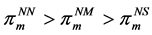

Proposition 6 characterizes the effects of the different power structures on the innovation investments. First, each firm’s innovation investment and profit are higher as the leader than as the follower. Moreover, the firm’s innovation investment and profit under the symmetric power structure are between those as the leader and as the follower if the innovation-desirability-index is lower, otherwise the highest.

The innovation decisions in the first stage are complementary, but the price decision in the second stage is substitute to each other. The two stages influence each other together to determine the performance of the supply chain. Proposition 6 shows, the leader of the supply chain gets more profits with higher innovation input (,) when they have little desire to innovate. When they have high desire to innovate, the chain members can get higher profits with higher innovation input using simultaneously-mover,

because the supplier and manufacturer’s profits increase in H (e.g., for the supplier, ,), and the marginal profit is larger by using simultaneously-mover than first- mover(e.g., for the supplier,).

In summary, under the non-cooperative innovation mode (N), it is optimal for a firm in the chain to cooperate with such a firm whose bargaining power is close to his own if the innovation-desirability-index is higher

, otherwise with such a firm whose bargaining power is lower to his own. Intuitively explaining,

the innovation-desirability-index, which is lower, means that innovation is more difficult and then innovation investment is large, so the chain members must use the first mover advantage to get more profits. Otherwise, innovation is more easy and then innovation investment is relatively little, so the members of the supply chain may give up the first mover advantage to promote innovation and then get more profits.

We now turn our attention to compare the different chain powers in sequence innovation. We take innovation scenario (S) as an example and get the following result.

Proposition 7. 1) For the innovation levels,

a) if,; otherwise,;

b) if,; otherwise,.

2) For the demand and chain profit, ,.

3) For the profits of the manufacture and the supplier,

a) if,; otherwise,;

b) if,; otherwise,.

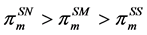Proposition 7 is similar to Proposition 6. When the supplier is the leader to invest in the first stage, each firm invests more in innovation and at the same time earns more as the leader than as the follower in the second stage. Under the symmetric chain power in the second stage, both firms’ investment in innovation and profits are between those as the leader and as the follower when H is not high, otherwise the largest one. The difference of Part 1) of Proposition 7 and Part 2) of Proposition 6 is that the cut-off points of the investments of the supplier and the manufacturer are similar in Part 1) Proposition 6, but are different in Part 2) of Proposition 7. Why?

From Table 1,. That means, the marginal growth rate of investment is identical

when the first stage is the non-cooperative innovation and the second stage is Nash-game. So the cut-off points

of investment of the two firms are identical. From Table 4, ,

. Then, we have. This means the marginal growth rate of

investment of the supplier is larger than the manufacturer when the first stage is the supplier leading sequential innovation and the second stage is Nash-game. So the cut-off point of supplier is little than the manufacturer’. Ditto we can explain the cut-off points of the profit of the supplier and the manufacturer are similar in Part 2) Proposition 6, but different in Part 3) of Proposition 7.

In summary, from Propositions 6 and 7, it is optimal in the chain to cooperate with such a firm whose bargaining power is close to his own for a firm if its innovation-desirability-index is higher, otherwise with such a firm whose bargaining power is lower to its own.

Based on the results summarized in Table 5, we can get the following interesting result.

Proposition 8. 1), , and.

2) If, and; otherwise and

.

Suppose both firms coordinate their innovation investments in the first stage. Then, the proposition tells us that each firm invests identically in innovation and the chain achieves the same demand and chain profit whether the supplier or the manufacturer is the leader in the second stage. However, each firm earns higher profit as the leader than as the follower in the second stage. Moreover, each firm’s profit in the symmetric chain power is between those as the leader and as the follower when H is not high (), otherwise the highest one.

The cut-off points of investment of the supplier and the manufacturer is not existed in Part 1) of Proposition 8, which is different to Part 2) of Proposition 7 and Proposition 6. Why? From Table 5, for the supplier,

,. It is obvious that. From Table 1, for the supplier, ,. It is obvious that and.

The cut-off points of profit of the supplier and the manufacturer is in Part 2) of Proposition 8, but in Part 2) of Proposition 6 and Part 3) of Proposition 7. Why are the cut-off points obviously large in Cooperative Innovation than in Non-Cooperative Innovation and Sequential Innovation? The investments of innovation are always no matter which H is, so the output can compensate the investment only when H is large enough.

In summary, it is optimal for a firm to cooperate with such a firm whose bargaining power is close to its own in the chain if the innovation-desirability-index is higher, otherwise with such a firm whose bargaining power is lower to its own.

5. Conclusions

In this paper, we have studied a supply chain where two firms first cooperate to invest on reducing component cost according to different modes and then compete for price according to different market powers. In the first stage (cooperative innovation stage), we consider the sequence of the investment decisions and the objective of the decision makers. In the second stage (price competition stage), we consider the sequence of the price decisions as three market powers of competition.

In the interaction between cooperative mode and market power, we focus on the firms’ choice of thr cooperative mode and the impact of market power on the firms’ decision. Our main findings are as follows. First, both the supplier and the manufacturer make more profits under mode M or S than under mode N given three structures of any market power. And, we show that the firms are easy to achieve cooperative innovation under symmetrical power market structure than under asymmetrical power market structure. Second, it is optimal for a firm in the chain to cooperate with such a firm whose market power is close to his own if the innovation- desirability-index is higher, otherwise with such a firm whose market power is lower to his own. Several research directions can follow from this study. First, we have not considered uncertainty in this framework. It would be interesting to consider the effects of demand uncertainty upon firms’ behavior. Second, it is worth studying firm behavior when the cost of the component information is asymmetric. Third, we have adopted the linear demand function, and it would be useful to examine whether the insights continue to hold for more general demand functions. Finally, it is also interesting to consider what will happen with competitive suppliers or competitive manufacturers.

Acknowledgements

We thank the Editor and the referee for their comments. The project was supported in part by the National Natural Science Foundation of China through Grants No. 71101082, and by Program for the Philosophy and Social Sciences Research of Higher Learning Institutions of Shanxi through Grants No. 2014305.

Cite this paper

SujuanWang,FangfangLiu, (2016) Cooperative Innovation in a Supply Chain with Different Market Power Structures. American Journal of Operations Research,06,173-198. doi: 10.4236/ajor.2016.62020

References

6. Appendix

6.1. Tables of Equilibria

6.2. Proofs of Propositions

The equilibrium under mode NS. We use backward induction to solve it. For any given and w, we can easily get the optimal retail price for the manufacturer in the last stage as follows:

Substituting it into, we get the optimal wholesale price by maximizing:

Thus, can be rewritten as a function of as follows

Substituting both and above into and, we get

By solving simultaneously the maximization problems and, we get the equilibrium innovation investment outputs:

Denote. We simplify and as

Therefore, the wholesale price, retail price, demand and profits of each member in equilibrium can be obtained. All are listed in column NS of Table 1.

The equilibria under other modes can be obtained similarly, and listed in Tables 1-5, respectively.

6.2.1. Proof of Proposition 1

We take as an example to prove the results. The proof for the other T is similar and omitted here. First we prove via the following results 1) to 4) from Table 1 and Table 2.

1). Then, since

.

2). Then, since

for.

3). So due to

for.

4). So due to

.

Next, we prove via the following results 1) to 4) from Table 1 and Table 2.

1). So, due to

.

2). So, due to

.

3). So since

.

4) So since

.

Finally, it is apparent that. This completes the proof.

6.2.2. Proof of Proposition 2

We take as an example to prove the proposition.

1) From Proposition 1, , and so. From Table 2 and Table 5,

Then, due to

. Again, It is

obvious that for

. As a result,.

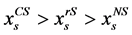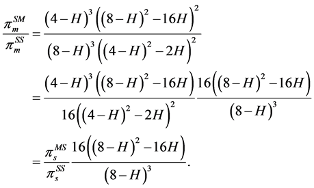
From Table 2 and Table 5, Then, if and only if

Note and

, due to. Since is strictly decreasing in,

So,. Again we have

Then, if and only if

due to. Hence,

.

2) From Table 2 and Table 5, So since

. Again from Table 2 and

Table 5, Then, due to

.

Next, from Table 1 and Table 2, So, due to

. Again from Table 1 and Table 2,

, and due to

. As a result,.

3) From Proposition 1, , , and so.

From Table 2 and Table 5, It is obvious that

if and only if, where

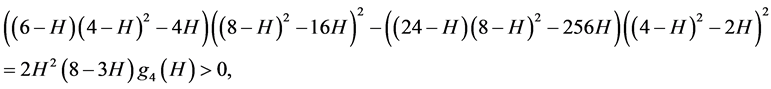
and. It suffices to show and. Now, for, and so is strictly decreasing in

. Thus, for. Moreover, and

. So, is strictly increasing in. Then,

for. Thus, is strictly decreasing in, and so for.

Again from Table 2 and Table 5, It is obvious that

if and only if

, where

. Now, and. So,

is strictly increasing in. Then, for, and so is strictly decreasing in. Therefore, for. This

completes the proof.

6.2.3. Proof of Proposition 3

We take as an example to prove the proposition. From Table 1 and Table 5, it is obvious that if and only if, or equivalently,

Denote by

. Then, the two roots of

equation are, respectively,

If, then is downward opening, and and. Thus, if, and so. Otherwise if, is upward opening. So,

. Now,

So, if, then and

. That is, if then, and if then.

As a result, if, or and, we then have. This completes the proof.

6.2.4. Proof of Proposition 4

The proofs of (i) and (ii) are identical.

(i) From Table 2,. It is apparent that if and only if

, where with

. Obviously, is strictly decreasing in, due to. Now,

, so.

Again from Table 2,. Then is equivalent to

which is true since.

From Table 2,

Then, since and.

Again from Table 2,. Then, is equivalent to

where. Now, and.

is strictly increasing in due to. Since,

for. Then is strictly decreasing in. Hence, due to

, for.

From Table 2,. Then, due to

.

Again from Table 2,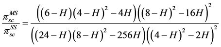. Then, if and only if

where. Now, and

. is strictly increasing in due to. Now,

, so for. Then is strictly decreasing in. Since, for. This completes the proof.

6.2.5. Proof of Proposition 5

From Table 4,. Furthermore,. It is apparent that

and if and only if which is true

due to.

From Table 4, it is obvious that and. This completes the proof.

6.2.6. Proof of Proposition 6

1) From Table 1, , so and. Similarly,

, so and. Again from Table 1,.

When, and, and so; Otherwise,.

2) From Table 1, , so and.

Similarly from Table 1, we have

due to for.

Again from Table 1,. Then and are equivalent

to

Now, and. So, is strictly decreasing in

, due to. Since, for. Then is strictly increasing in. Hence, due to, , and so there is an unique such that for but for. We get an

approximate solution by solving a cubic equation. This completes the proof.

6.2.7. Proof of Proposition 7

1.a) and 3.a) From Table 2 and Table 3, It is apparent that and

if and only if Since

, is strictly decreasing in. Now, , so

for.

From Table 3 and Table 4,. It is apparent that and

if and only if. Since

, is strictly decreasing in. Now, , so for.

From Table 2 and Table 4,. Then, and if and

only if Since

, is strictly increasing in. Now, and , so for otherwise.

1.b) From Table 2 and Table 3,. Then, due to

From Table 2 and Table 4,. So, if and only if

Since

, is strictly decreasing in. Now, , so for.

From Table 3 and Table 4,. So, if and only if

. Since

, is strictly increasing in. Now, , , so for otherwise.

2) From Table 2 and Table 3, , if. From Propositions 4,. From

Table 3 and Table 4,. It is apparent that if and only if

. This is equivalent to

. Since, is strictly decreasing in. Now, , so for.

From Table 2 and Table 3, , if. From Propositions 4,. From Table 3 and Table 4,

It suffices to show

, which is

equivalent to. Now,

is strictly increasing in. Now, , is strictly decreasing in

due to for. Since and

, there is an unique such that for otherwise

. That is, is strictly decreasing in, but strictly increasing in. So is a unimodal function. Now, and, so. That is, is strictly increasing in. Due to, for. That is, is strictly decreasing in. Now, , so for.

3.b) From Table 2 and Table 3,

It is apparent that if and only if

. Since

and. is strictly decreasing in. Now, , so is strictly decreasing in due to for. Due to , for.

From Table 2 and Table 4, Then, if and only if

. Now,

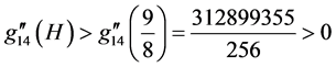So, is strictly decreasing in. Now, , is strictly increasing in. Then, , is strictly decreasing in. So, for. That is, is strictly

increasing in. Thus, , and so is strictly decreasing in. Therefore, for.

From Table 3 and Table 4, It is apparent that if and

only if. Now,

So, is strictly increasing in. This implies that and so is strictly decreasing in. This together with implies that is strictly increasing in. Now, , so is strictly decreasing in. Since and, there is an unique such that for but otherwise. That is, is strictly decreasing in, but strictly increasing in. Now, , so

for. Moreover,. There is an unique such that for but otherwise. We get an approximate

solution by solving a six order equation. This completes the proof.

6.2.8. Proof of Proposition 8

1) From Table 5, it is obvious that, , , , and

, , and.

2) From Table 5, and. It is apparent that

and if and only if, which is true due

to.

Again from Table 5, since

. This completes the proof.

6.3. Necessity of Condition (SOC) for the Existence of Equilibria

The SOC of mode N under different market power:

1) About the equilibrium of mode (NS), the profit is a quadratic function of and. So, it is necessary to require

At the same time, is required to ensure. All the three conditions are ensured by.

2) In mode (NM), the profit is a quadratic function of and. So, it is necessary to require

At the same time, is required to ensure. All the three conditions are ensured by.

3) In mode (NN), the profit is a quadratic function of and. So, it is necessary to require

At the same time, is required to ensure. All the three conditions are ensured by.

The SOC of mode S and M under different market power:

4) In mode (SS), when the efforts of the supplier are observed by the manufacturer, the profit is a quadratic function of and. So it is necessary to require

Then, the profit is a quadratic function of and. So it is necessary to require

Both of the two conditions are ensured by and.

5) In mode (MS), when the efforts of the manufacturer are observed by the supplier, the profit is a quadratic function of and. So it is necessary to requir

Then, the profit is a quadratic function of and. So it is necessary to require

Both of the two conditions are ensured by and.

6) In mode (SM), the profit is a quadratic function of and. So it is necessary to requir

and

7) In mode (MM), the profit is a quadratic function of and. So it is necessary to require

and

8) In mode (SN), the profit is a quadratic function of and. So it is necessary to require

and

9) In mode (MN), the profit is a quadratic function of and. So it is necessary to require

and

The SOC of mode C under different market power:

10) In mode (CM, CS), the profit is a quadratic function of and. Then, we require the negativity of the Hessian matrix of with respect to and. This is equivalent to, after some algebraic computations, that

That is, , and, all of which are ensured by.

11) In mode (CN), the profit is a quadratic function of and. Then, we require the negativity of the Hessian matrix of with respect to and. This is equivalent to, after some algebraic computations, that

That is, , and, all of which are ensured by.

It is apparent that the second order conditions above are always true whenever. If,

.

References

- 1. Jeffrey, L.Y. and Thomas, C. (2004) Building Deep Supplier Relationships. Harvard Business Review, 82, 104-113.
- 2. Choi, S.C. (1991) Price Competition in a Channel Structure with a Common Retailer. Marketing Science, 10, 271-297.
http://dx.doi.org/10.1287/mksc.10.4.271 - 3. Trivedi, M. (1998) Distribution Channels: An Extension of Exclusive Retailership. Management Science, 44, 896-909.
http://dx.doi.org/10.1287/mnsc.44.7.896 - 4. Wu, C.H., Chen, C.W. and Hsieh, C.C. (2012) Competitive Pricing Decisions in a Two-Echelon Supply Chain with Horizontal and Vertical Competition. International Journal of Production Economics, 135, 265-274.
http://dx.doi.org/10.1016/j.ijpe.2011.07.020 - 5. Aberdeen, G. (2006) The Product Lifecycle Collaboration Benchmark Report: The Product Profitability “X Factor”? Aberdeen Group, Boston.
- 6. Levin, R.C. and Reiss, P.C. (1988) Cost-Reducing and Demand-Creating R&D with Spillovers. Rand Journal of Economics, 19, 538-556.
http://dx.doi.org/10.2307/2555456 - 7. Brown, M. and Svenson, R. (1988) Measuring R&D Productivity. Research Technology Management, 31, 11-15.
http://dx.doi.org/10.1016/j.respol.2004.07.003 - 8. Belderbos, R., Carree, M. and Lokshin, B. (2004) Cooperative R&D and Firm Performance. Research Policy, 33, 1477-1492.
- 9. Stallkamp, T.T. (2005) SCORE! A Better Way to Do Business: Moving from Conflict to Collaboration. Wharton School Publishing, Upper Saddle River.
- 10. Gupta, S. and Loulou, R. (1998) Process Innovation, Product Differentiation, and Channel Structure: Strategic Incentives in a Duopoly. Marketing Science, 17, 301-316.
http://dx.doi.org/10.1287/mksc.17.4.301 - 11. Gupta, S. (2008) Channel Structure with Knowledge Spillovers. Marketing Science, 27, 247-261.
http://dx.doi.org/10.1287/mksc.1070.0285 - 12. Gilbert, S.M. and Cvsa, V. (2003) Strategic Commitment to Price to Stimulate Downstream Innovation in a Supply Chain. European Journal of Operational Research, 150, 617-639.
http://dx.doi.org/10.1016/S0377-2217(02)00590-8 - 13. Bernstein, F. and Kök, A.G. (2009) Dynamic Cost Reduction through Process Improvement in Assembly Networks. Management Science, 55, 552-567.
http://dx.doi.org/10.1287/mnsc.1080.0961 - 14. Bhaskaran, S.R. and Krishnan, V. (2009) Effort, Revenue, and Cost Sharing Mechanisms for Collaborative New Product Development. Management Science, 55, 1152-1169.
http://dx.doi.org/10.1287/mnsc.1090.1010 - 15. Kim, S.H. and Netessine, S. (2013) Collaborative Cost Reduction and Component Procurement. Management Science, 59, 189-206.
http://dx.doi.org/10.1287/mnsc.1120.1573 - 16. Ishii, A. (2004) Cooperative R&D between Vertically Related Firms with Spillovers. International Journal of Industrial Organization, 22, 1213-1235.
http://dx.doi.org/10.1016/j.ijindorg.2004.05.003 - 17. Ge, Z., Hu, Q. and Xia, Y. (2014) Firms’ R&D Cooperation Behavior in a Supply Chain. Production & Operations Management, 23, 599-609.
http://dx.doi.org/10.1111/poms.12037 - 18. Messinger, P.R. and Narasimhan, C. (1995) Has Power Shifted in the Grocery Channel? Marketing Science, 14, 189-223.
http://dx.doi.org/10.1287/mksc.14.2.189 - 19. Raju, J.Z. and Zhang, J. (2005) Channel Coordination in the Presence of a Dominant Retailer. Marketing Science, 24, 254-262.
http://dx.doi.org/10.1287/mksc.1040.0081 - 20. Iyer, G. and Villas-Boas, J.M. (2003) A Bargaining Theory of Distribution Channels. Journal of Marketing Research, 40, 80-100.
http://dx.doi.org/10.1509/jmkr.40.1.80.19134 - 21. Dukes, A.J., Gal-Or, E. and Srinivasan, K. (2006) Channel Bargaining with Retailer Asymmetry. Journal of Marketing Research, 4, 84-97.
http://dx.doi.org/10.1509/jmkr.43.1.84 - 22. Lu, J.C., Tsao, Y.C. and Charoensiriwath, C. (2011) Competition under Manufacturer Service and Retail Price. Economic Modelling, 28, 1256-1264.
http://dx.doi.org/10.1016/j.econmod.2011.01.008 - 23. Ertek, G. and Griffin, P.M. (2002) Supplier- and Buyer-Driven Channels in a Two-Stage Supply Chain. IIE Transactions, 34, 691-700.
http://dx.doi.org/10.1080/07408170208928905 - 24. Zhang, R., Liu, B. and Wang, W.L. (2012) Pricing Decisions in a Dual Channels System with Different Power Structures. Economics Modeling, 29, 523-533.
http://dx.doi.org/10.1016/j.econmod.2011.08.024 - 25. Wei, J., Zhao, J. and Li, Y. (2013) Pricing Decisions for Complementary Products with Firms’ Different Market Powers. European Journal of Operational Research, 224, 507-519.
http://dx.doi.org/10.1016/j.ejor.2012.09.011 - 26. Amir, R. and Stepanova, A. (2006) Second-Mover Advantage and Price Leadership in Bertrand Duopoly. Games and Economic Behavior, 55, 1-20.
http://dx.doi.org/10.1016/j.geb.2005.03.004 - 27. Ba’rcena-Ruiz, J.C. (2007) Endogenous Timing in a Mixed Duopoly: Price Competition. Journal of Economics, 91, 263-272.
http://dx.doi.org/10.1007/s00712-007-0255-5 - 28. Granot, D. and Yin, S. (2007) On Sequential Commitment in the Price-Dependent Newsvendor Model. European Journal of Operational Research, 177, 939-968.
http://dx.doi.org/10.1016/j.ejor.2006.01.013 - 29. Su, M. and Rao, V.R. (2011) Timing Decisions of New Product Preannouncement and Launch with Competition. International Journal of Production Economics, 129, 51-64.
http://dx.doi.org/10.1016/j.ijpe.2010.09.001 - 30. Gurnani, H., Erkoc, M. and Luo, Y. (2007) Impact of Product Pricing and Timing of Investment Decisions on Supply Chain Co-Opetition. European Journal of Operational Research, 180, 228-248.
http://dx.doi.org/10.1016/j.ejor.2006.02.047 - 31. D’Aspremont, C. and Jacquemin, A. (1988) Cooperative and Noncooperative R&D in Duopoly with Spillovers. American Economic Review, 78, 1133-1137.
- 32. Kamien, M., Muller, E. and Zang, I. (1992) Research joint ventures and R&D Cartels. American Economic Review, 82, 1293-1306.
- 33. Ge, Z. and Hu, Q. (2008) Collaboration in R&D Activities: Firm-Specific Decisions. European Journal of Operational Research, 185, 864-883.
http://dx.doi.org/10.1016/j.ejor.2007.01.020 - 34. Dyer, J.H. and Hatch, N.W. (2006) Relation-Specific Capabilities and Barriers to Knowledge Transfers: Creating Advantage through Network Relationships. Strategic Management Journal, 27, 701-719.
http://dx.doi.org/10.1002/smj.543 - 35. Dyer, J.H. and Nobeoka, K. (2000) Creating and Managing a High Performance Knowledge Sharing Network: The Toyota Case. Strategic Management Journal, 21, 345-367.
http://dx.doi.org/10.1002/(SICI)1097-0266(200003)21:3<345::AID-SMJ96>3.0.CO;2-N