ABSTRACT

Multiple objective stochastic linear programming is a relevant topic. As a matter of fact, many practical problems ranging from portfolio selection to water resource management may be cast into this framework. Severe limitations on objectivity are encountered in this field because of the simultaneous presence of randomness and conflicting goals. In such a turbulent environment, the mainstay of rational choice cannot hold and it is virtually impossible to provide a truly scientific foundation for an optimal decision. In this paper, we resort to the bounded rationality principle to introduce satisfying solution for multiobjective stochastic linear programming problems. These solutions that are based on the chance-constrained paradigm are characterized under the assumption of normality of involved random variables. Ways for singling out such solutions are also discussed and a numerical example provided for the sake of illustration.

1. Introduction

Decision makers are intendedly rational. They are goal directed and they are intended to pursue those goals in conformity with the classic homo-economicus model [1]. They do not always succeed because of the complexity of some environments that impose both procedural and substantive limits. This is the case when dealing with multiobjective stochastic linear programming (MSLP) problems.

In such a turbulent environment the notion of “optimum optimorum” is not clearly defined and satisficing rather than optimal search behavior seems to be the most appropriate option. A look at the literature reveals that most existing solution concepts for MSLP problems rely heavily on the expected, pessimistic and optimistic values of involved random variables [2,3]. A finding from several research work [4-7] leave no doubt about the fact that these values may be useful in providing the range of possible outcomes. Nevertheless, they ignore such important factors as the size and the probability of deviations outside the likely range as well as other aspects concerning the dispersion of the probabilities.

In this paper, we discuss satisfying solution concepts for MSLP problems. These concepts are based on the chance-constrained philosophy [8]. Chance-constrained applied for the purpose of limiting the probability that constraint will be violated. In this form, it adds considerably to both the flexibility and reality of the stochastic model under consideration. Mathematical characterization of the above mentioned solution concepts are also provided along with ways for singling them out. A numerical example is supplemented for the sake of illustration.

The remainder of the paper is organized as follows. In the next section we clearly formulate the problem under consideration. In Section 3, we present some satisfying solution concepts for this problem. In Section 4, we characterize these solution concepts. In Section 5, we discuss ways for solving resulting problems. In Section 6, we present the methods for solving this problem. An illustrative example is given in Section 7. We end up with some concluding remarks along with lines for further developments in the field of MSLP.

2. Multiobjective Stochastic Linear Programming

Problem Formulation

A multiobjective stochastic linear programming is a problem of the following type:

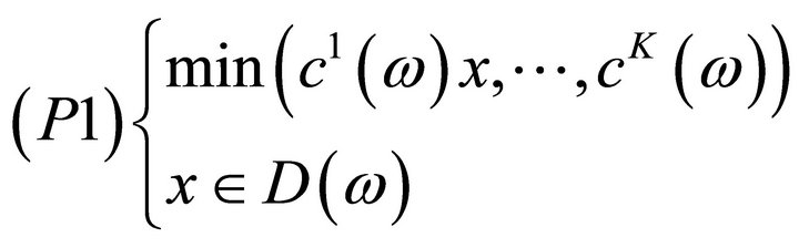
where 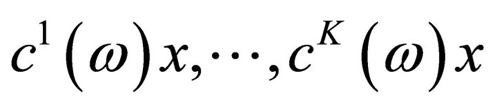are random vectors defined on a probability space,

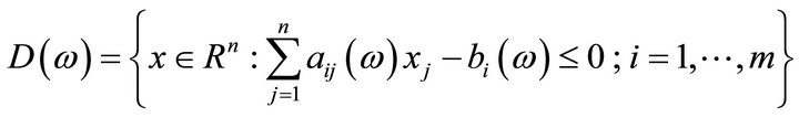
where are random variables defined on the same probability space.

(P1) is an ill-defined problem because of the simultaneous presence of different objective functions and of randomness surrounding data. In such a turbulent environment, neither the notion of feasibility nor that of optimality is clearly defined. One then has to resort to the Simon’s bounded rationality principle [9] and seek for a satisfying solution instead of an optimal one.

Several solution concepts have been described in the literature, see for instance [10,11]. Most of these solution concepts rely on the first two moments of involved random variables. As mentioned earlier, these values often offer a short-sighted view of uncertainty surrounding data under consideration. In what follows, we discuss some satisfying solution concepts based on the chanceconstrained approach [12-14].

3. Satisfying Solutions for Problem (P1)

Definition 3.1 -satisfying solution of type 1 Assume that objective functions of (P1) are aggregated in the form of. We say that is an -satisfying solution of type 1 for if is optimal for the following optimization problem:

where with and and β are probability levels a priori fixed by the Decision Maker.

Definition 3.2 -satisfying solution of type 2 We say that is an -satisfying solution of type 2 for (P1) if, where, is efficient for the following multiobjective optimization problem:

Here and are threshold fixed by the Decision Maker.

Definition 3.3 -satisfying solution of type 3 We say that is an -satisfying solution of type 3 for (P1) if, where, is optimal for the following mathematical program:

Here, and are respectively the upper deviations of the goal, the weight of and the target associated with the objective function. and are as in Definition 3.2.

Interpretation

Intuitive ways of thinking about the above solution concepts are given below.

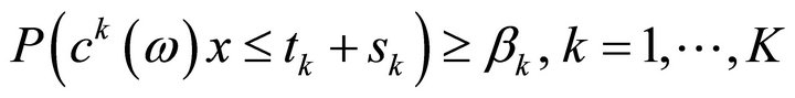
• An -satisfying solution of type 1 for is an alternative that keeps the probability of the aggregate of the objective functions of this problem, lower than a variable s to a desired extend β, while the variable s is itself minimized. Moreover the chance of meeting the constraint of the problem is requested to be higher than fixed thresholds. It is clear that for and β close to 1, such an alternative is an interesting one. As a matter of fact, it maintains the probability of keeping the aggregation of objective functions low, while keeping the probabilities of realization of constraints to desired extents.

• An -satisfying solution of type 2 for is an action that keeps the probability of the objective of the problem be less than some variable to a level: while the vector is minimized in the Pareto sense. In the meantime, the chance of having the constraint of the problem be satisfied is greater than. Again for, and, close to 1, such a solution is interesting from the stand points of feasibility and efficiency.

• Finally, an -satisfying solution of type 3 for minimizes the weighted sum of derivations from given targets while maintaining the probability of each objective to be close to the corresponding target, to some desired levels. It also meets the requirement of being feasible with high probability.

4. Characterization of Satisfying Solutions

In what follows, we provide necessary and sufficient conditions for a potential action to be a satisfying one, in the above described sense. These conditions rely heavily on the hypothesis of normality of distributions of involved random variables.

We recall that random vector is said to have the multivariate normal distribution if any linear combination of its components is normally distributed. The following Lemma due to Kataoka [13] will be needed in the sequel.

Lemma 4.1

1) Assume that are independent and normally distributed random variables with mean

respectively.

Then for, the aggregation 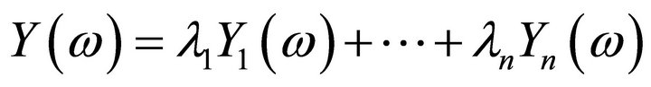is normally distributed with mean

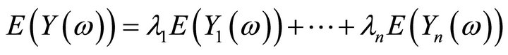
and variance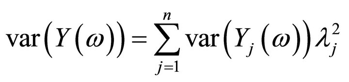

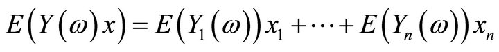
2) Suppose has a multivariate normal distribution with mean

and let be the covariance of and Then for any, the inner product 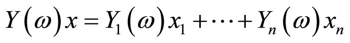is normally distributed with mean

and variance

.

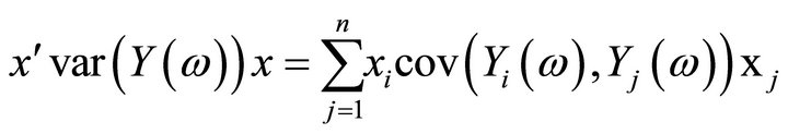We are now in position to characterize an - satisfying solution of type 1.

Proposition 4.1

Assume that objective functions of (P1) is aggregated as follows 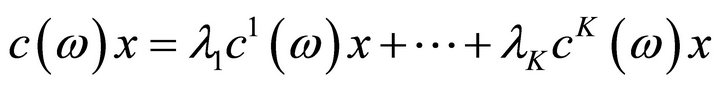where,

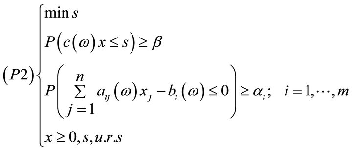
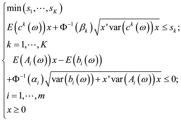
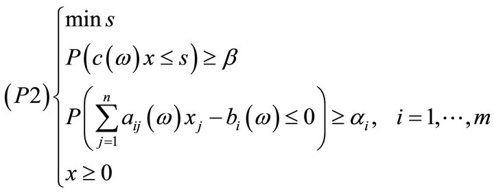
, Suppose that the random variables,; are independent and normally distributed. Suppose also that for any, the random variables and are normally distributed and independent. Then a point is an -satisfying solution of type 1 for (P1) if and only if is optimal for the problem:

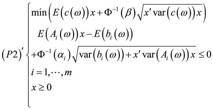
where, , denotes the row of the matrix and

Proof

Assume that is a satisfying solution of type 1 for (P1), then is a solution of

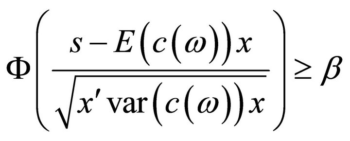
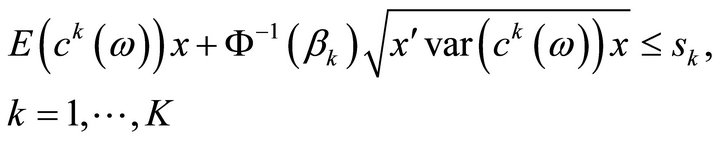
Let’s show that the first constraint of (P2) is equivalent to

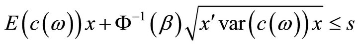(1)

Indeed we have by Lemma 4.1 that is normally distributed with mean and variance .

Then

because

is normally distributed with mean 0 and variance 1. Therefore the first constraint of becomes

That is

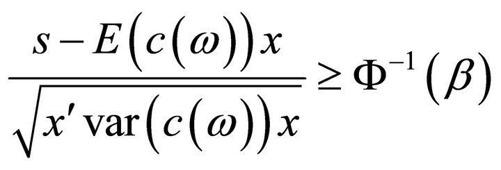
which equivalent is to:

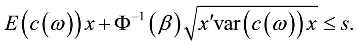
And we have established that the first constraint of

is equivalent to relation (1).

Define now the random variables

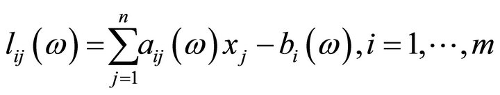
are independent and normally distributed [15].

The expected value of is

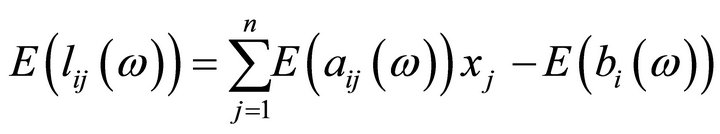(2)

and its variances is

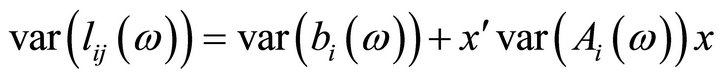. (3)

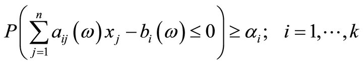
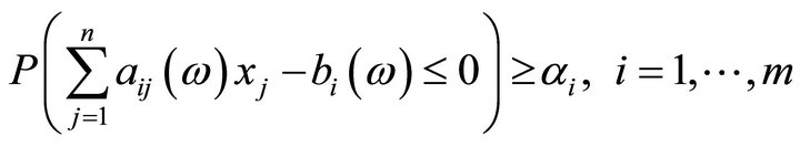
The chance constraints

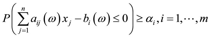(4)

can therefore, be written as

;

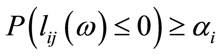which can also be expressed as

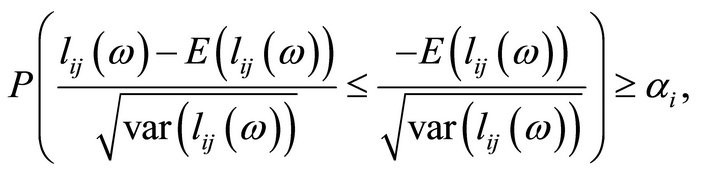
or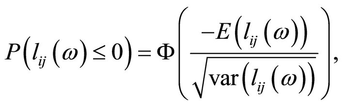        

where

Thus the chance constraints (4) can be merely written:

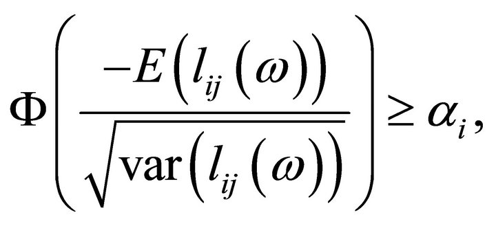
that is

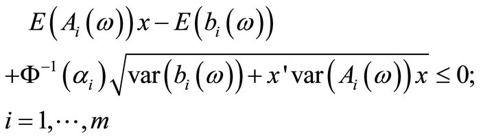
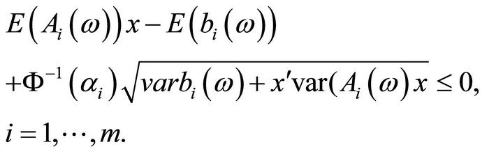
which leads to replacing and by their values given by (2) and (3) respectively in (4), we obtain

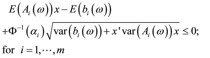(5)

combining relations (1) and (5) we obtain that is optimal to the following program:

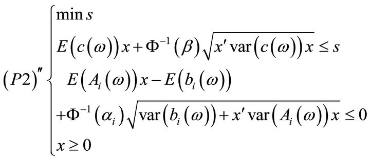
This problem is equivalent to (P2)' as desired.

As far as -satisfying solution of type 2 is concerned we have the following result.

Proposition 4.2

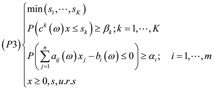
Consider (P1) and assume that the random variables ; are independent and normally distributed. Assume further that the random variables;; and; are also normally distributed and independent. Then a point is an -satisfying solution of type 2 for (P1) if and only if is efficient for the following mathematical program:

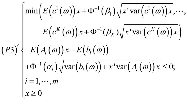
where; and denotes the row of the matrix and

.

Proof

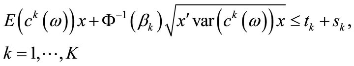
As shown in the proof of Proposition 4.1, the chance constraints 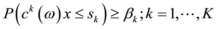in (P3) are equivalent to

and the chance constraints:

are equivalent to

Then (P3) is equivalent to the following program:

And clearly, this problem is equivalent to (P3)' in the sense that they have the same efficient solutions. Finally, a characterization of an -satisfying solution of type 3 is given below.

Proposition 4.3

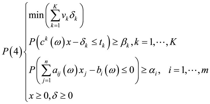
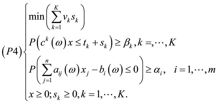
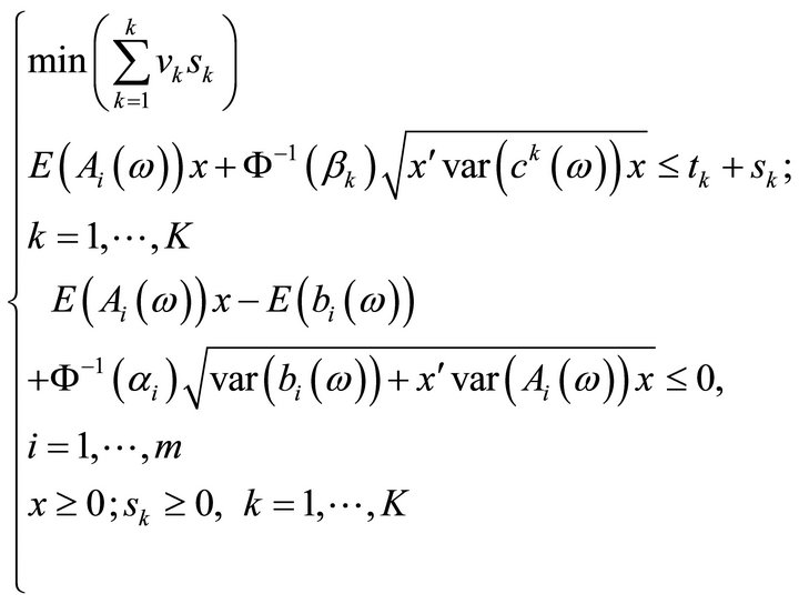
Consider (P1) and assume that the random variables,; are independent and normally distributed. Then a point is an -satisfying solution of type 3 for problem (P1) if and only if is optimal for the following mathematical program:

where is the upper deviation variable of the goal, are weights of the upper deviation variables, are targets associated with the objective functions; denotes the row of the matrix 

and, are desired thresholds fixed by the Decision Maker.

Proof.

Consider

As discussed in the proof of Proposition 4.2, the chance constraints

are equivalent to

As shown in the proof of Proposition 4.1, we have that

can be written as follow:

Therefore, program reads:

which is exactly (P4)'.

5. Singling out Satisfying Solution for Problem (P1)

Problem to be solved to single out a satisfying solution (in the sense of definitions given in, §2 for (P1) are (P2)', (P3)' and (P4)' depending on the type of solution chosen. (P2)' and (P4)' are standard mathematical programs about which a great deal is known. In the case, when these programs are convex, one may use algorithms of convex programming [16], the conjugate gradient method [17], the exterior or interior penalty functions methods [18]. For the non convex case, one may use approximation type algorithms or metaheuristics [19]. (P3)' is a multiobjective program. A rich array of methods for solving it may be found in [20].

6. Methods for Solving (P1)

6.1. Method for Yielding a Satisfying Solution of Type 1

Step 1: Fix and; ;

Step 2: Compute;;

Step 3: Compute;

Step 4: Agregate to;

Step 5: Compute, , ,;

Step 6: Write the Program;

Step 7: Solve using a mathematical programming method. Let is solution;

Step 8: Print: “is a satisfying solution of type1 for (P1)”;

Step 9: Stop.

6.2. Method for Yielding a Satisfying Solution of Type 2

The same as 6.1; except that in Step 1 should be replaced by

In Step 4, should be replaced by and, respectively.

Steps 5-7 should be as follow:

Step 5: Write the Program;

Step 6: “Solve” and in;

Step 7, “is a satisfying solution of type 2”;

Step 8: Stop.

6.3. Method for Yielding a Satisfying Solution of Type 3

Step 1: Fix and;

Step 2: Fix, and,;

Step 3: Compute:, , ,;

Step 4: Compute:,; , , , ,;

Step 5: Write;

Step 6: Solve let its solution;

Step 7: Print: “is a satisfying solution of type 3”;

Step 8: Stop.

7. Numerical Example

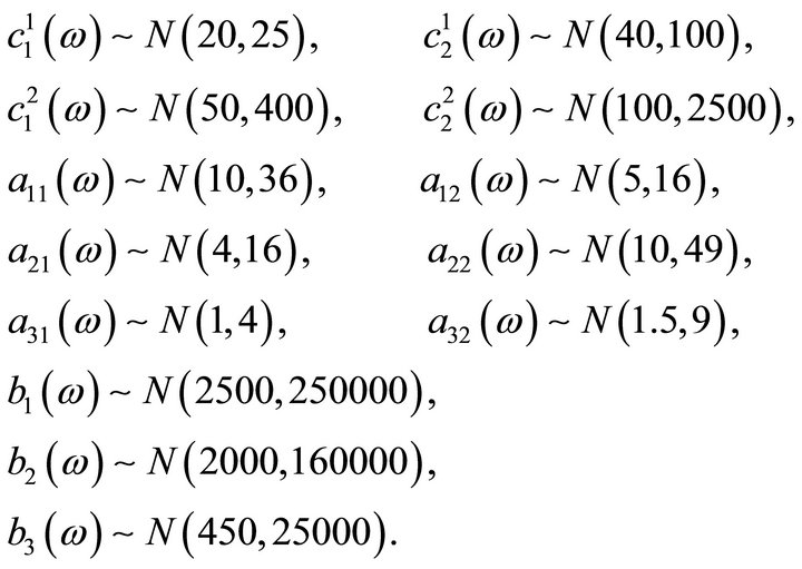
Consider the following multiobjective stochastic linear program:

where, are independent normally distributed random variables, with the following parameters:

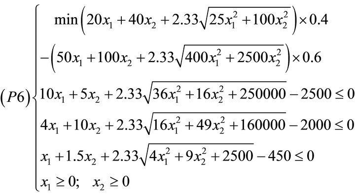
if the decision maker is interested in a satisfying solution of type 1 with and and then by virtue of Proposition 4.1, he has to solve the following problem.

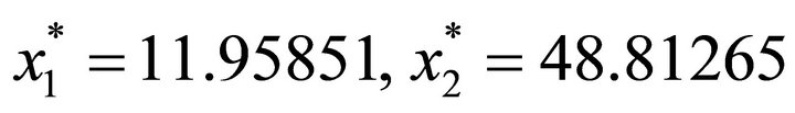
solving this optimization problem using MATLAB, we obtain the following solution:

.

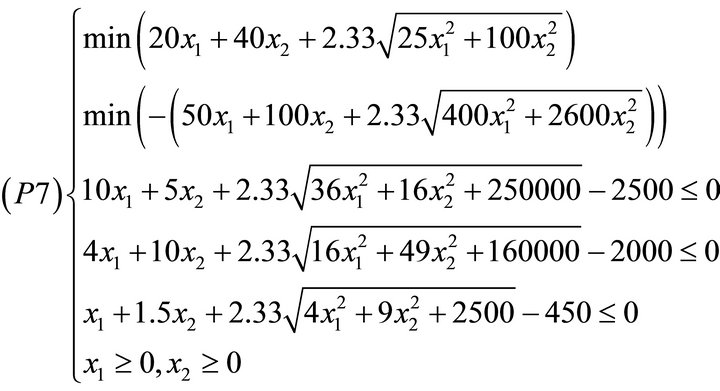
Assume now that a satisfying solution of type 2 is sought with and .

Then by Proposition 4.2, one has to solve the following problem:

using the global criterion method [21] and solving the resulting problem by MATLAB, we obtain the following solution:

Suppose that a satisfying solution of type 3 is desirable for and 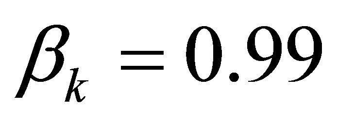. Suppose further that the decision maker goals are 2,000 and 15,000 for objectives 1 and 2 respectively. Using equal weights (i.e. 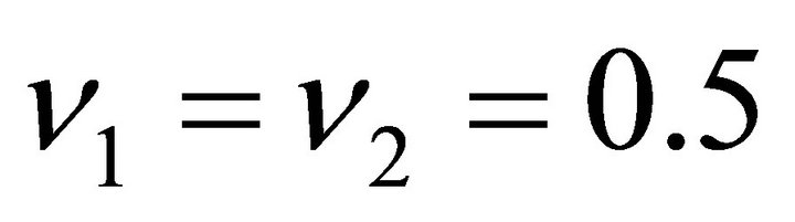for the two objectives, we have to solve the following problem:

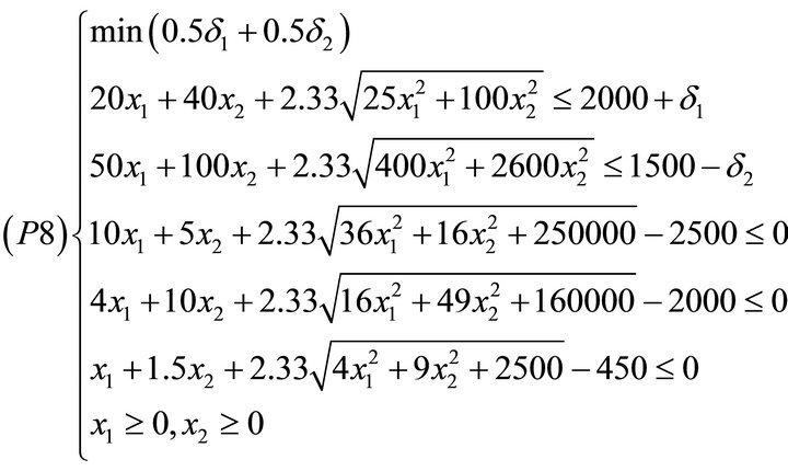
using MATLAB to solve this problem, we obtain the following solution:, , , with optimal value .

As can be seen, methods yielding type 2 and type 3 satisfying solutions have almost the same solution that differs from the method yielding type 1 solution satisfying solution. This is because the two first methods use the multiobjective approach while the third method uses the stochastic approach.

8. Concluding Remarks

In this paper, we have addressed the problems of defining and characterizing solution concepts for a multiobjective stochastic linear program. Owing to the simultaneous presence of randomness and to the multiplicity of objective functions, we have privileged the satisfying approach rather than the optimizing one.

Solution concepts discussed in this paper have an advantage over those focusing only on the expectation and variances. As a matter of fact, these solutions take into consideration, the whole distributions of involved random variables. We have shown that when involved random variables are normally distributed, singling out solutions discussed here causes little extra computational costs. As a matter of fact, problems to be solved to obtain such solutions are standard mathematical programs about which a great deal is known. Lines for further developments in this field include:

• The choice of threshold, , and, in an optimal way;

• The consideration of other distributions rather than the normal one;

• The extension of solution concepts discussed here to the case where fuzziness and randomness are in the state of affairs [22];

• The generalization of methods discussed here to the bilevel case [23].

REFERENCES

- P. C. Fishburn, “Utility for Decision Making,” John Wiley, New York, 1970.
- R. Caballero, E. Cerdà, M. M. Munoz and L. Rey, “Relations among Several Efficiency Concepts in Stochastic Multiple Objective Programming,” In: Y. Y. Haines and R. E. Steuer, Eds., Research and Practice in Multiple Criteria Decision Making, 2000.
- R. Caballero, E. Cerdà, M. M. Muñoz, L. Rey and I. M. “Stancu-Minasian, Efficient Solution Concepts and Their Relations in Stochastic Multiobjective Programming,” Journal of Optimization Theory and Applications, Vol. 110, No. 1, 2001, pp. 53-74. doi:10.1023/A:1017591412366
- P. Rietveld and H. Ouwersloot, “Ordinal Data in Multicriteria Decision Making, a Stochastic Dominance Approach to Sitting Nuclear Power Plants,” European Journal of Operational Research, Vol. 56, No. 2, 1992, pp. 249-262. doi:10.1016/0377-2217(92)90226-Y
- H. M. Markowitz, “Mean Variance Analysis in Portfolio choice and Capital Markets,” Basil Blackwell, Oxford, 1970.
- B. Liu, “Theory and Practice of Uncertainly Programming,” Physical-Verley, Heidelberg, 2002.
- A. S. Adeyefa and M. K. Luhandjula, “Multiobjective Stochastic Linear Programming: An Overview,” American Journal of Operations Research, Vol. 1, No. 4, 2011, pp. 203-213. http://www.SciRP.org/journal/ajor
- A. Charnes and W. W. Cooper, “Chance-Constrained Programming,” Management Science, Vol. 6, No. 1, 1959, pp. 73-79. doi:10.1287/mnsc.6.1.73
- H. A. Simon, “A Behavior Model of Rational Choice,” In: Models of Man: Social and Rational, Macmillan, New York, 1957.
- I. M. Staincu-Minasian, “Overview of Different Approaches for Solving Stochastic Programming Problems with Multiple Objective Functions,” In: S.-Y. Huang and J. Teghem, Eds., Stochastic versus Fuzzy Approaches to Multiobjective Mathematical Programming under Uncertaintly, Kluwer Academic Publisher, Dordrecht, 1990.
- I. M. Stancu-Minasian, “Stochastic Programming with Multiple Objective Functions,” D. Reidel Publishing Company, Boston, 1984.
- P. Kall, “Stochastic Linear Programming,” Springer-Verlag, Berlin, 1972.
- S. Kataoka, “A Stochastic Programming Model,” Econometrica, Vol. 31, No. 1-2, 1963, pp. 181-196.
- B. Liu, “Introduction to Uncertain Programming,” Tsinghua University, Beijing, 2005. (Unpublished)
- J. K. Sengupta, “Stochastic Programming: Methods and Applications,” North-Holland Publishing Company, Amsterdam, 1972.
- G. P. McCormick and K. Ritter, “Methods of Conjugate Directions versus Quasi-Newton Methods,” Mathematical Programming, Vol. 3, No. 1, 1972, pp. 101-116
- R. Flecher and C. M. Reeves, “Function Minimization by Conjugate Gradients,” The Computer Journal, Vol. 7, No. 2, 1964, pp. 149-154. doi:10.1093/comjnl/7.2.149
- J. P. Evans, F. J. Gould and J. W. Tolle, “Exact Penalty Functions in Nonlinear Programming,” Mathematical Programming, Vol. 4, No. 1, 1973, pp. 72-79. doi:10.1007/BF01584647
- A. K. Bhunia and J. Majumda, “Elitist Genetic Algorithm for Assignment Problem with Imprecise Goal,” European Journal of Operational Research, Vol. 177, No. 2, 2007, pp. 684-692. doi:10.1016/j.ejor.2005.11.034
- K. M. Miettinem, “Nonlinear Multiobjective Optimization,” Kluwer Academic Publishers, Massachusetts, 1999.
- B. C. Eaves and W. I. Zangwill, “Generalized Cutting Plane Algorithms,” SIAM Journal on Control, Vol. 9, No. 4, 1971, pp. 529-542. doi:10.1137/0309037
- M. K. Luhandjula, “On Fuzzy Random-Valued Optimization,” American Journal of Operations Research, Vol. 1, No. 4, 2011, pp. 259-267. doi:10.4236/ajor.2011.14030
- C. P. Olivier, “Solving Bilevel Linear Multiobjective Programming Problems,” American Journal of Operations Research, Vol. 1, No. 4, 2011, pp. 214-219.