World Journal of Engineering and Technology
Vol.05 No.04(2017), Article ID:79542,9 pages
10.4236/wjet.2017.54B005
Velocity Decomposition Method for Ship Advancing in Calm Water Simulation
Ji Zhao, Renchuan Zhu, Guoping Miao
State Key Laboratory of Ocean Engineering, Collaborative Innovation Center for Advance Ship and Deep-Sea Exploration, Shanghai Jiao Tong University, Shanghai, China


Received: August 3, 2017; Accepted: October 9, 2017; Published: October 12, 2017
ABSTRACT
In this study, a viscous-inviscid method based on velocity decomposition is presented. The velocity of the flow field is decomposed into viscous velocity and inviscid velocity, the inviscid velocity is applied for the whole domain, which includes the damping area, and the remaining viscous velocity is just acting on a small domain around the ship hull according to the boundary layer theory. The remaining viscous velocity is computed by a modified N-S equation which coupled the inviscid part, after the inviscid velocity is obtained by solving Euler equation. The simulation of Wigley hull advancing in calm water is accomplished with present method also the decomposed velocity has been studied. The result shows the present method is robust and can be a practical method for partial viscous correction.
Keywords:
Inviscid/Viscous, Modified N-S Equation, Velocity Decomposition, Wigley Hull

1. Introduction
For the simulation of ship advancing in the calm water, the shape of free surface and the wave making force can be obtained accurately with the assumption of potential flow [1] [2] [3], and the viscous effect can be corrected with empirical formula estimation. Because according to Prandtl’s boundary layer theory, the viscous just effects around the body surface and the far field can be treated as potential flow. Based on this point, calculating the shape of free surface and far field with the inviscid assumption and do the viscous correction around the ship hull shall be a wise choice.
Thus far, there has been many researches in coupling viscous and inviscid flow [4] [5] [6], and the viscous/inviscid method have been widely applied for many hydrodynamic problems. This method always accomplished by decomposing the flow domain and iterating on the interface of viscous and inviscid domain, however these methods are not able to do the partial viscous correction, that the inviscid field has obtained already and need to correct the areas with significant viscous effects.
The main purpose of our present work is to develop a practical and efficient solver for viscous correction and ship hydrodynamic problems simulation. In this work, a velocity decomposition [7] method for simulating the Wigley hull advancing in the calm water is presented in detail. The present method is programmed on the platform of OpenFOAM and the solver is applicable for simulating the cases with free surfaces. The simulation of Wigley hull advancing in calm water has been completed with both velocity decomposition method and the traditional CFD method, the result agreed well with the experiment data, which shows the present method is suitable for viscous correction and ship hydrodynamic simulation.
2. Theory of the Viscous/Inviscid Method
The simulation of ship advancing in the calm water is a popular case in the area of ship hydrodynamic, and the govern equations can be written as follow,
(1)
where is the velocity of the flow field; p is pressure; ν is viscosity; is water phase fraction; express as , is water density and is air density; S is a source term including the gravity source, free surface tension source and damping source.
Generally, the viscous has little contribute to the shape of free surface, because the wave making resistance and free surface shape can be obtained by potential theory exactly. Here we ignore the viscous and free surface tensor, the govern equation of inviscid velocity can be written as
(2)
(3)
where is the coming flow velocity, is a damping coefficient, x0 and x1 are the horizontal coordinates of the damping zone boundary.
As to the area around the ship hull, the viscous effect cannot be ignored. Mostly, the ITTC equation is supposed to be used for the drag force correction, while it is not accurate enough in many situations. To obtain a better viscous correction, here we decompose the total velocity into inviscid velocity and viscous velocity .
(4)
For the calculating of the viscous velocity, a much smaller domain size can be used according to boundary layer theory as shown in Figure 1, so the damping zone is not include in the viscous zone obviously, and the source term can be omitted.
The free surface of ship advancing can be treated as quasi steady state, so the phase need not to be calculated again, and the density can be treated as constant. With these assumption, substituting (4) into govern Equation (1), we can get the modified NS equation for the viscous velocity as bellow.
(5)
Equation (5) is the govern equation for the viscous velocity, which coupled the inviscid velocity. The Equation (5) keeps the form of NS equation, but much simple than the original form, so it is supposed to be a fast and accurate way for the viscous correction.
3. Numerical Implantation Method
3.1. Domain Decomposition
Before solving the modified N-S equation, the inviscid velocity in the viscous zone should be obtained first according to (5). Generally, the inviscid zone and the viscous zone uses different set of meshes, and to obtain the inviscid velocity, the interpolation cannot be avoided. However, the velocity interpolation including the boundary surface and the interior zone shall take much time, and the computation efficient can be effected, so the domain decomposition is also adopted here.

Figure 1. Sketch of viscous and inviscid domain.
The domain decompose method is showed in Figure 2. When solving the inviscid velocity, zone 1 and zone 2 are combined. Then the inviscid velocity in viscous zone can be obtained by mapping without interpolation. At last the viscous velocity can be solved in zone 2 with its boundary condition showed below.
3.2. Boundary Condition
The viscous velocity is obtained by solving modified N-S equation after the inviscid velocity is obtained, and the solving process is nearly the same with the traditional CFD method while the boundary condition have some obvious differences (Table 1).
Where the OpenFOAM solvers LTSinterFoam is adopt as CFD method for solving turbulence and laminar flow respectively. For the velocity boundary, the biggest difference locates at the body B.C. and the inlet B.C. For the truncated boundary, the viscous velocity is used zero value B.C. instead of fixed value of U for the assumption that the flow at the truncated position can be treated as potential flow. The body B.C. is derived from the no-slip boundary condition, so the sum of potential velocity and non-potential velocity should be zero.
For the outlet boundary, the boundary condition should be the same as the inlet B.C. according to the velocity decomposition theory, while it will cause continuity errors during the solution. Besides the outlet boundary contains a part of wake zone, where the viscous effect cannot be ignored, so the flow at the outlet boundary cannot be treated as potential flow and a zero gradient B.C. is used.

Figure 2. Sketch of domain decompose method.

Table 1. Boundary condition.
The k and omega boundary value are calculated with the formula below:
; (6)
where U is the flow velocity, I is Turbulence intensity, l is Turbulence length scale. It is worth to mention that when the pressure decomposed, the pressure B.C for the body should be changed to negative potential pressure gradient.
4. Results
The simulation of Wigely hull advance in the calm water is famous in the ship hydrodynamic area, and there is enough experiment data and simulation result for comparison, so it is good to be chosen to test the velocity decomposition theory. The shape of the Wigley hull can be express as:
(7)
where L = 1 m is the length of the hull, B = 0.1 m is the hull width, T = 0.0625 m is the draft. As the computation domain is decomposed as mentioned before, the range of the inviscid domain and the viscous domain are showed in Table 2 and Figure 3.
The k-omega SST model is adopted in the computing of the viscous velocity, so the mesh in the viscous zone should be dense enough for the simulation. The average y+ is chosen 100, the mesh of the inviscid and viscous domain are shown as follow Figure 4 and Figure 5.

Figure 3. Sketch of viscous and inviscid domain.
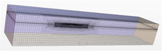
Figure 4. Mesh of the inviscid domain.

Figure 5. Mesh of the viscous domain.
Table 2. Domain size.
According to the velocity decomposition theory, the final velocity field is the summation of inviscid velocity field and the viscous velocity field. So, it is necessary to export these flow fields for further study.
Figures 6-9 give the velocity count by traditional CFD method u, the velocity result by velocity decomposition method ut, the inviscid velocity by velocity decomposition method up, the viscous velocity by viscous/inviscid method u* respectively.
In the viscous velocity counter of Figure 7, the velocity in the far field except the wake zone and some area of free surface is almost zero which means the computation domain can be reduced and the present velocity decomposition method can capture the area of viscous effects. Also the viscous velocity on the free surface is zero in most area means the viscous contributes little to the free surface.
Figure 10 gives the wave height along the Wigley hull, from this figure it is clear that there exist some difference in the front and after of the Wigley hull, where the viscous effect is obvious. However, the wave height calculated with inviscid assumption correspond with experiment data [8] very well, which means it is reasonable to compute the free surface with the assumption of inviscid.
It is clear that the drag force cannot be computed correctly if the viscous been ignored, so the result of drag force shall be a good criterion to judge the velocity decomposition method.
The drag force and its component at Fr = 0.32 are shown in Table 3, and the results are agreed well with the experiment data. From the table, it is obvious that the velocity decomposition method is even turned to be a little better than the CFD method, which means that the present method is robust and accurate for viscous correction.
5. Conclusions
To accomplish the simulation of the ship advance in the calm water, a velocity decomposition method is presented in this work. In this method, the fluid is treated inviscid in a large domain which include the damping zone and the viscous is considered in a small domain with some reasonable assumption. The simulation of ship advancing in calm water is completed by present method. Through analyzing the result of cases, it can be concluded as follow.
Firstly, the present velocity decomposition method is suitable for simulating the ship advancing in calm water. The drag force result calculated by present method agrees with the experiment data very well, which proves that the present

Figure 6. Velocity count of ue by present method.

Figure 7. Velocity count of u* by present method.

Figure 8. Velocity count of ut by present method.

Figure 9. Velocity count of u by traditional CFD method.

Figure 10. The comparison of wave profile on the hull at Fr = 0.32.
Table 3. Force coefficient at Fr = 0.32.
method is robust and the assumption in this work is reasonable.
Secondly, the present velocity decomposition method is efficient in viscous correction and numerical simulation. In the present, if the inviscid flow field is obtained advance, the result that considered viscous can be obtained fast by solving the modified N-S equation in a small domain easily, so it is a good method for partial viscous correction. Also, this method can be treated as a viscous-inviscid coupling method for simulation.
Last, the present velocity decomposition method can reflect the viscous effect in the flow domain. In the viscous velocity count, the viscous effect is positive correlation with magnitude of viscous velocity, and which result is helpful to study the viscous effect.
Cite this paper
Zhao, J., Zhu, R.C. and Miao, G.P. (2017) Velocity Decomposition Method for Ship Advancing in Calm Water Simulation. World Journal of Engineering and Technology, 5, 42-50. https://doi.org/10.4236/wjet.2017.54B005
References
- 1. Chen, X., Zhu, R.C., Miao, G.P., et al. (2015) Calculation of Ship Sinkage, Trim and Wave Drag Using High-Order Rankine Source Method. Shipbuilding of Chi-na, No. 3, 1-12.
- 2. Chen, X., Zhu, R.C., Ma, C., et al. (2016) Computations of Linear and Nonlinear Ship Waves by Higher-Order Boundary Element Method. Ocean Engineering, 114, 142-153. https://doi.org/10.1016/j.oceaneng.2016.01.016
- 3. Shao, Y.-L. (2010) Numerical Potential-Flow Studies on Weakly-Nonlinear Wave-Body Interactions with/without Small Forward Speeds. Norwegian University of Science and Technology, Norway, 43-44.
- 4. Dinh, Q.V., Glowinski, R., Périaux, J., et al. (1988) On the Coupling of Viscous and Inviscid Models for Incompressible Fluid Flows via Domain Decomposition. In: Glowinski, R., Golub, G., Meurant, G., et al., Eds., First International Symposium on Domain Decomposition Methods for Partial Diferential Equations, SIAM, Philadelphia, 350-369.
- 5. Hamilton, J.A. (2002) Viscous-Inviscid Matching for Wave-Body Interaction Problems. Univer-sity of California, Berkeley.
- 6. Purohit, J.B. (2013) An Improved Vis-cous-Inviscid Interactive Method and Its Application to Ducted Propel-lers.
- 7. Helmholtz, H. (1867) LXIII. On Integrals of the Hydrodynamical Equations, Which Express Vortex-Motion. The London, Edinburgh, and Dublin Philosophical Magazine and Journal of Science, 33, 485-512.
- 8. Kajitani, H., Miyata, H., Ikehata, M., et al. (1983) The Summary of the Cooperative Experi-ment on Wigley Parabolic Model in Japan.
- 9. Sangseon, J. (1983) Study of Total and Viscous Resistance for the Wigley Parabolic Ship Form.