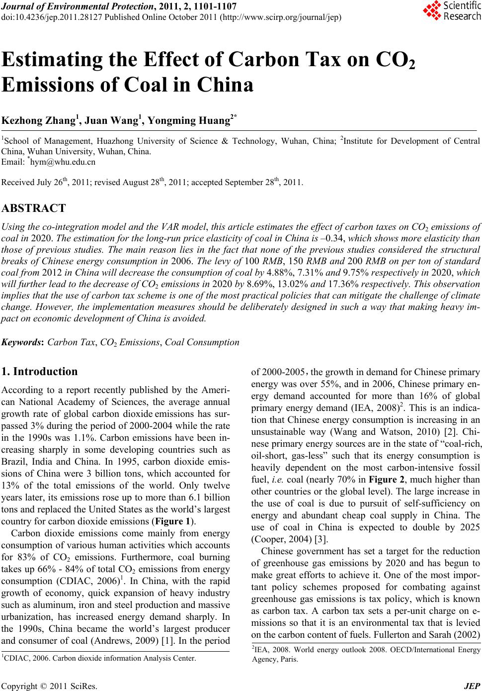
Journal of Environmental Protection, 2011, 2, 1101-1107
doi:10.4236/jep.2011.28127 Published Online October 2011 (http://www.scirp.org/journal/jep)
Estimating the Effect of Carbon Tax on CO2
Emissions of Coal in China
Kezhong Zhang1, Juan Wang1, Yongming Huang2*
1School of Management, Huazhong University of Science & Technology, Wuhan, China; 2Institute for Development of Central
China, Wuhan University, Wuhan, China.
Received July 26th, 2011; revised August 28th, 2011; accepted September 28th, 2011.
ABSTRACT
Using the co-integration model and the VAR model, this article estimates the effect of carbon taxes on CO2 emissions of
coal in 2020. The estimation for the long -run price elasticity of coal in China is –0.34, which shows more elasticity tha n
those of previous studies. The main reason lies in the fact that none of the previous studies considered the structural
breaks of Chinese energy consumption in 2006. The levy of 100 RMB, 150 RMB and 200 RMB on per ton of standard
coal from 2012 in China will decrease the consumption of coal by 4.88%, 7.31% and 9.75% respectively in 2020, whic h
will further lead to the decrease of CO2 emissions in 2020 by 8.69%, 13.02% and 17.36% respectively. This observation
implies that the use of carbon tax scheme is one of the most practical policies that can mitigate the challenge of climate
change. However, the implementation measures should be deliberately designed in such a way that making heavy im-
pact on economic development of China is avoided.
Keywords: Carbon Tax, CO2 Emissions, Coal Consumption
1. Introduction
According to a report recently published by the Ameri-
can National Academy of Sciences, the average annual
growth rate of global carbon dioxide emissions has sur-
passed 3% during the period of 2000-2004 while the rate
in the 1990s was 1.1%. Carbon emissions have been in-
creasing sharply in some developing countries such as
Brazil, India and China. In 1995, carbon dioxide emis-
sions of China were 3 billion tons, which accounted for
13% of the total emissions of the world. Only twelve
years later, its emissions rose up to more than 6.1 billion
tons and replaced the United States as the world’s largest
country for carbon dioxide emissions (Figure 1).
Carbon dioxide emissions come mainly from energy
consumption of various human activities which accounts
for 83% of CO2 emissions. Furthermore, coal burning
takes up 66% - 84% of total CO2 emissions from energy
consumption (CDIAC, 2006)1. In China, with the rapid
growth of economy, quick expansion of heavy industry
such as aluminum, iron and steel production and massive
urbanization, has increased energy demand sharply. In
the 1990s, China became the world’s largest producer
and consumer of coal (Andrews, 2009) [1]. In the period
of 2000-2005，the growth in demand for Chinese primary
energy was over 55%, and in 2006, Chinese primary en-
ergy demand accounted for more than 16% of global
primary energy demand (IEA, 2008)2. This is an indica-
tion that Chinese energy consumption is increasing in an
unsustainable way (Wang and Watson, 2010) [2]. Chi-
nese primary energy sources are in the state of “coal-rich,
oil-short, gas-less” such that its energy consumption is
heavily dependent on the most carbon-intensive fossil
fuel, i.e. coal (nearly 70% in Figure 2, much higher than
other countries or the global level). The large increase in
the use of coal is due to pursuit of self-sufficiency on
energy and abundant cheap coal supply in China. The
use of coal in China is expected to double by 2025
(Cooper, 2004) [3].
Chinese government has set a target for the reduction
of greenhouse gas emissions by 2020 and has begun to
make great efforts to achieve it. One of the most impor-
tant policy schemes proposed for combating against
greenhouse gas emissions is tax policy, which is known
as carbon tax. A carbon tax sets a per-unit charge on e-
missions so that it is an environmental tax that is levied
on the carbon content of fuels. Fullerton and Sarah (2002)
2IEA, 2008. World energy outlook 2008. OECD/International Energy
Agency, Paris.
1CDIAC, 2006. Carbon dioxide information Analysis Center.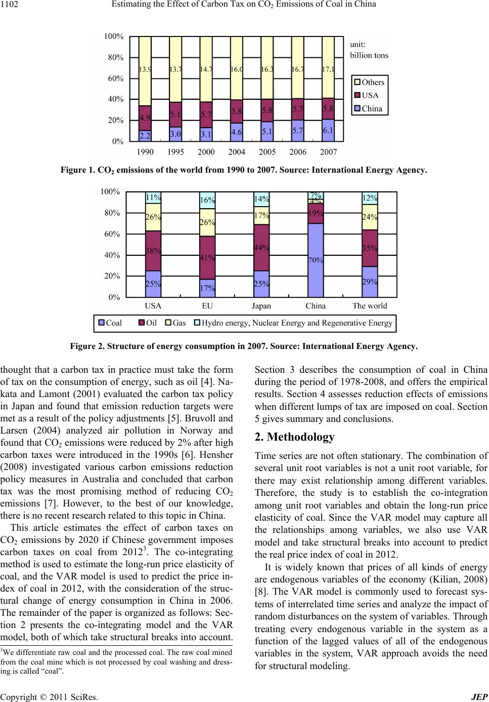

Estimating the Effect of Carbon Tax on CO Emissions of Coal in China 1102 2
Figure 1. CO2 emissions of the world from 1990 to 2007. Source: International Energy Agency.
Figure 2. Structure of energy consumption in 2007. Source: International Energy Agency.
thought that a carbon tax in practice must take the form
of tax on the consumption of energy, such as oil [4]. Na-
kata and Lamont (2001) evaluated the carbon tax policy
in Japan and found that emission reduction targets were
met as a result of the policy adjustments [5]. Bruvoll and
Larsen (2004) analyzed air pollution in Norway and
found that CO2 emissions were reduced by 2% after high
carbon taxes were introduced in the 1990s [6]. Hensher
(2008) investigated various carbon emissions reduction
policy measures in Australia and concluded that carbon
tax was the most promising method of reducing CO2
emissions [7]. However, to the best of our knowledge,
there is no recent research related to this topic in China.
This article estimates the effect of carbon taxes on
CO2 emissions by 2020 if Chinese government imposes
carbon taxes on coal from 20123. The co-integrating
method is used to estimate the long-run price elasticity of
coal, and the VAR model is used to predict the price in-
dex of coal in 2012, with the consideration of the struc-
tural change of energy consumption in China in 2006.
The remainder of the paper is organized as follows: Sec-
tion 2 presents the co-integrating model and the VAR
model, both of which take structural breaks into account.
Section 3 describes the consumption of coal in China
during the period of 1978-2008, and offers the empirical
results. Section 4 assesses reduction effects of emissions
when different lumps of tax are imposed on coal. Section
5 gives summary and conclusions.
2. Methodology
Time series are not often stationary. The combination of
several unit root variables is not a unit root variable, for
there may exist relationship among different variables.
Therefore, the study is to establish the co-integration
among unit root variables and obtain the long-run price
elasticity of coal. Since the VAR model may capture all
the relationships among variables, we also use VAR
model and take structural breaks into account to predict
the real price index of coal in 2012.
It is widely known that prices of all kinds of energy
are endogenous variables of the economy (Kilian, 2008)
[8]. The VAR model is commonly used to forecast sys-
tems of interrelated time series and analyze the impact of
random disturbances on the system of variables. Through
treating every endogenous variable in the system as a
function of the lagged values of all of the endogenous
variables in the system, VAR approach avoids the need
for structural modeling.
3We differentiate raw coal and the processed coal. The raw coal mined
from the coal mine which is not processed by coal washing and dress-
ing is called “coal”.
C opyright © 2011 SciRes. JEP

Estimating the Effect of Carbon Tax on CO Emissions of Coal in China1103
2
Price is usually assumed as the basic variable which
determines coal demand. In some other literatures, such
as Dahl, Carol, Thomas Sterner (1991) [9], Kilian (2008),
Bento, Goulder, Jacobsen and Roger (2009) [10], GDP
was assumed as another macroeconomic controlled vari-
able. Our model takes price and GDP as the main factors
affecting the demand for coal. Besides, we also treat the
consumption of oil as the controlled variable since it is
an alternative for coal. In order to eliminate the factor of
population expansion, we use per capita consumption
and per capita GDP. There are four kinds of data: per
capita consumption of coal, the fixed basic price index of
coal in real terms, real per capita GDP, and per capita
consumption of oil. All these variables are in logarithm
form and denoted t, t, t and t respectively.
It is easy to know the coefficient of is the price elas-
ticity of coal.
lc lp lg lo
t
lp
Furthermore, we use the dummy variable

to define
the vital event concerning structural changes of energy
consumption in the sample from 1978 to 2012. The State
Council of the People’s Republic of China formally
promulgated the first document for energy conservation
in 2006, which explicitly announced the preferential
taxation policies for energy saving. The taxation policy is
a useful and efficient tool to promote energy saving and
reduce pollution, and is often used to modify firm be-
havior, especially in developing countries (Sivadasan and
Slemrod, 2008) [11]. As coal will become more expen-
sive in the long run, a lot of firms and households may
adjust their demand for coal or choose some “cheaper
and renewable” fuel as alternatives. Thus, we have



0,1978, 2005
1,2006, 2012
t
t





where denotes the time point of structural
change, and [ ] denotes the period. The co-integrating
equation used in this paper is
2006=t
01 23 4tttt
lclp lg lot

     (1)
where t

is the residual and all the data for variables
are annual.
In order to test the property of each variable in the data,
which is the order of integrating of the variables of
Equation (1), we use the PP test and KPSS test to deter-
mine the stationary of four variables t, t, t and
t. The null hypothesis of PP test is non-stationary,
while the null hypothesis of KPSS test is stationary. Af-
ter estimating Equation (1), the unit root test is applied to
the residual series
lc lplg
lo
t

as shown in Equation (2)
11
1
ˆˆ ˆ
k
tt it
i
where ˆt

is the estimated residual of Equation (1), k is
the number of lags making-up the residuals of Equation
(2) to approximate a white noise process, and （if
1k
1k

, 00


）.
Subsequently, taking the structural change as exoge-
nous variable, we use the residual-based co-integrating to
examine whether all the variables have a stable relation-
ship in a long term. Remark that all the variables should
have the same order of integration in order to do the
co-integrating regression. In this paper, the unit root tests
indicate all variables that will be presented in the next
section have the same order of integration. Some other
studies have proved that there exists a co-integrating
relationship between energy demand and macroeconomic
variables for gasoline demand in Denmark (Bentzen,
2004) [12] and for gasoline demand in India (Ramana-
than, 1999) [13]. If the residual series are stationary at a
level after applying the unit root test, then we reject the
hypothesis of ˆ=0

. The test statistics of Johansen
co-integrating mainly have Trace Statistic. The null hy-
pothesis of Trace Statistic means that the number of
co-integrating equation(s) is r, otherwise, it is . The
formula is
k


1
ln 1
k
tr i
ir
LRr kT



 
 (3)
where i

is the i-th characteristics root of a matrix ar-
rayed in descending sequence.
Then, the VAR model is used and the structural
change is treated as exogenous variable to predict the
price index of coal in 2012. The reduced form of VAR (q)
model is
11tt ptpt
yAyAyDx t



  (4)
where is a vector of time series, 1t y×1K,,
q
A
A
are ×
K
K matrices of coefficients to be estimated, t
x
is a vector of exogenous variables, is the coefficients
of exogenous variables and t
D

is vector of in-
novations and unobservable zero mean white noise proc-
ess which is also called forecast error. t
×1K

may be con-
temporaneously correlated but are uncorrelated with their
own lagged values and uncorrelated with all variables in
the right-hand side.
The same logic applies in the more general VAR (p)
model that allows for additional unrestricted delayed
feedback among per capital coal consumption and its
price index, per capital GDP, per capital oil consumption.
All the variables are modified corresponding to a lagged
order . Where , and
p

,,,
ttttt
ylclplglo



1234
,,,
ttttt



. Then, the structural form of the
t

 


 
 (2) VAR (p) model is as follows: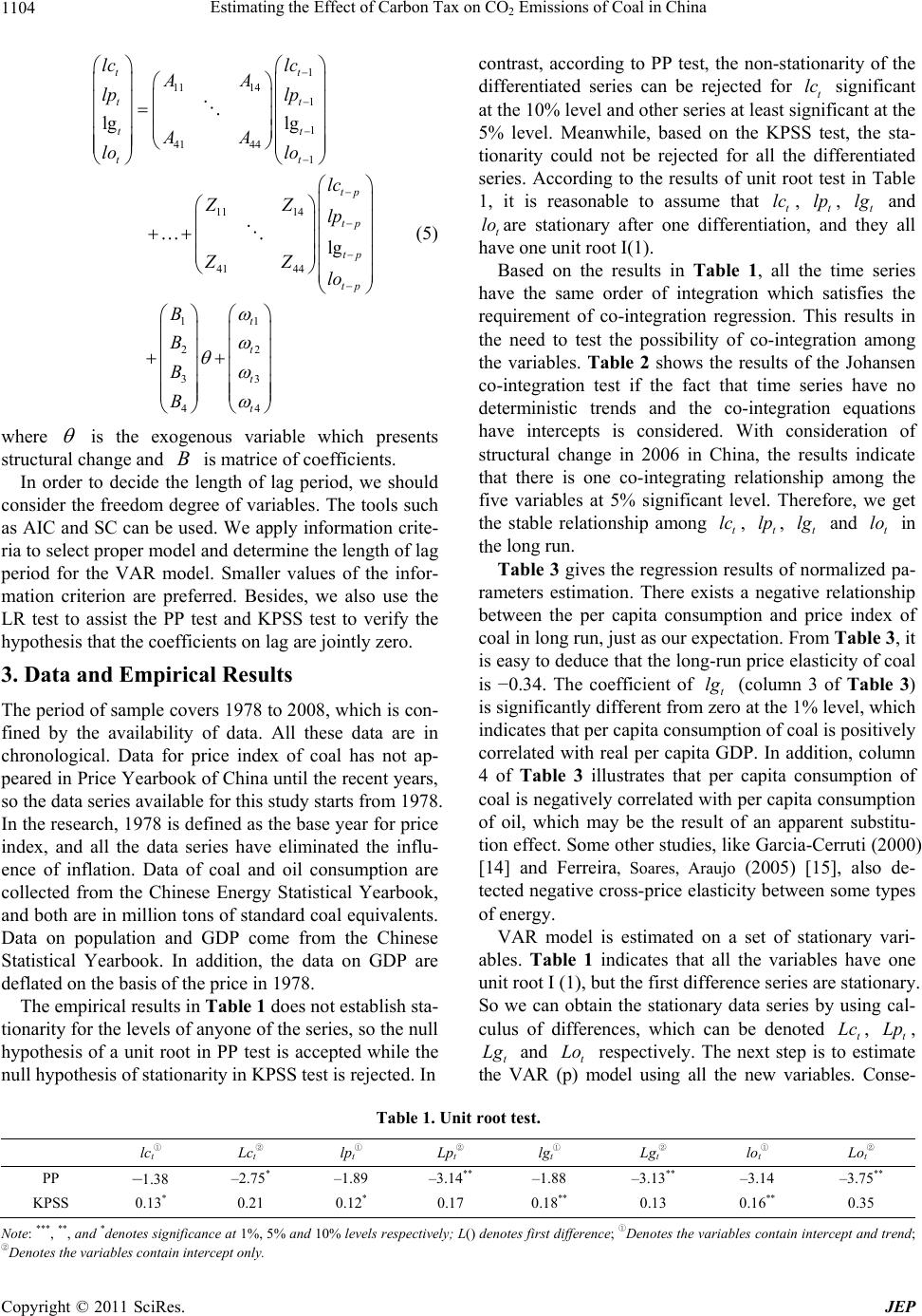

Estimating the Effect of Carbon Tax on CO2 Emissions of Coal in China 1104


1
11 14
1
1
41 44
1
11 14
41 44
1 1
2 2
33
44
lg lg
lg
tt
tt
tt
tt
tp
tp
tp
tp
t
t
t
t
lc lc
AA
lp lp
AA
lo lo
lc
ZZ
lp
ZZ
lo
B
B
B
B












 

 

 

 

 

 
 





 







 
 


  

 
 

 (5)
contrast, according to PP test, the non-stationarity of the
differentiated series can be rejected for t significant
at the 10% level and other series at least significant at the
5% level. Meanwhile, based on the KPSS test, the sta-
tionarity could not be rejected for all the differentiated
series. According to the results of unit root test in Table
1, it is reasonable to assume that t, t, t and
tare stationary after one differentiation, and they all
have one unit root I(1).
lc
lplc lg
lo
Based on the results in Table 1, all the time series
have the same order of integration which satisfies the
requirement of co-integration regression. This results in
the need to test the possibility of co-integration among
the variables. Table 2 shows the results of the Johansen
co-integration test if the fact that time series have no
deterministic trends and the co-integration equations
have intercepts is considered. With consideration of
structural change in 2006 in China, the results indicate
that there is one co-integrating relationship among the
five variables at 5% significant level. Therefore, we get
the stable relationship among , , and in
the long run.
t
lc t lp t lg t lo
where

is the exogenous variable which presents
structural change and
B
is matrice of coefficients.
In order to decide the length of lag period, we should
consider the freedom degree of variables. The tools such
as AIC and SC can be used. We apply information crite-
ria to select proper model and determine the length of lag
period for the VAR model. Smaller values of the infor-
mation criterion are preferred. Besides, we also use the
LR test to assist the PP test and KPSS test to verify the
hypothesis that the coefficients on lag are jointly zero.
Table 3 gives the regression results of normalized pa-
rameters estimation. There exists a negative relationship
between the per capita consumption and price index of
coal in long run, just as our expectation. From Table 3, it
is easy to deduce that the long-run price elasticity of coal
is −0.34. The coefficient of t (column 3 of Table 3)
is significantly different from zero at the 1% level, which
indicates that per capita consumption of coal is positively
correlated with real per capita GDP. In addition, column
4 of Table 3 illustrates that per capita consumption of
coal is negatively correlated with per capita consumption
of oil, which may be the result of an apparent substitu-
tion effect. Some other studies, like Garcia-Cerruti (2000)
[14] and Ferreira, Soares, Araujo (2005) [15], also de-
tected negative cross-price elasticity between some types
of energy.
lg
3. Data and Empirical Results
The period of sample covers 1978 to 2008, which is con-
fined by the availability of data. All these data are in
chronological. Data for price index of coal has not ap-
peared in Price Yearbook of China until the recent years,
so the data series available for this study starts from 1978.
In the research, 1978 is defined as the base year for price
index, and all the data series have eliminated the influ-
ence of inflation. Data of coal and oil consumption are
collected from the Chinese Energy Statistical Yearbook,
and both are in million tons of standard coal equivalents.
Data on population and GDP come from the Chinese
Statistical Yearbook. In addition, the data on GDP are
deflated on the basis of the price in 1978.
VAR model is estimated on a set of stationary vari-
ables. Table 1 indicates that all the variables have one
unit root I (1), but the first difference series are stationary.
So we can obtain the stationary data series by using cal-
culus of differences, which can be denoted t, t,
t and t respectively. The next step is to estimate
the VAR (p) model using all the new variables. Conse-
Lc Lp
Lg Lo
The empirical results in Table 1 does not establish sta-
tionarity for the levels of anyone of the series, so the null
hypothesis of a unit root in PP test is accepted while the
null hypothesis of stationarity in KPSS test is rejected. In
Table 1. Unit root test.
lct① Lct② lpt① Lpt② lgt① Lgt② lot① Lot②
PP –1.38 –2.75* –1.89 –3.14** –1.88 –3.13** –3.14 –3.75**
KPSS 0.13* 0.21 0.12* 0.17 0.18** 0.13 0.16** 0.35
Note: ***, **, and *denotes significance at 1%, 5% and 10% levels resp ectively; L() denotes first difference; ①Denotes the variables contain intercept and trend;
②Denotes the variables contain intercept only.

Estimating the Effect of Carbon Tax on CO Emissions of Coal in China1105
2
Table 2. Johansen co-integration test.
Hypothesized
no. of CE(s)
Trace
statistic
0.05
critical value Prob.**
r = 0 58.51* 47.86 0.00
r ≤ 1 18.76 29.80 0.51
r ≤ 2 8.85 15.49 0.38
Note: *Denotes rejection of the null hypothesis at the 0.05 significance level;
**Denotes MacKinnon Haug Michelis (1999) p-values; the series have no
deterministic t rends but have intercepts.
Table 3. Results of co-integrating.
Variables lpt lgt lot constant
Coefficient –0.34 1.90*** –1.70*** –7.52
Standard error 0.42 0.65 0.38
Adj. R-squared 0.67
Note: ***, **, and *denote significance at 1%, 5% and 10% levels r espec-
tively.
quently, we also determine the lagged length of the
model. The VAR (p) model consists of a system of equa-
tions that express each variable as a linear function of its
own lagged value and the lagged values of all the other
variables in the system. The VAR (p) model is used to fit
to the data, and the AIC, SC and LR criterions are used
as the first approach to develop the optimal lagged length.
At last, we conduct diagnostics tests on the residuals of
each equation, and adjust the lagged length in order to
guarantee the statistical validity of the model and the
simultaneous maximization of the freedom degrees
(Ferreira, Soares and Araujo, 2005). The test results sug-
gest p = 1 for the model. The VAR (1) model is shown as
follows:
1
1
1
1
1.150.150.43 0.14
0.290.54 0.49 0.24
0.240.05 0.980.05
0.17 0.150.17 0.84
0.10 0.29
0.05 4.83
0.04 1.45
0.09 0.07
t
tt
tt
t
t t
Lc lc
Lp lp
Lg lg
lo
Lo





 

 

 


 


 

 
















(6)
Equation (6) gives estimated parameters of the VAR
(1) model, by which we can estimate the values of t
from 1978 to 2003 and obtain the value of t. In Fig-
ure 3, the pink line describes the predicted results of t
from 1978 to 2003 while the blue line describes the real
results. Then we predict the results of t from 2004 to
2008 and obtain the value of t. Some better fitting
prediction of t are in Table 4. Note worthily, the re-
sults in Table 4 illustrate the deviation between the real
Lp
lp
lp
Lp
lp
lp
and predicted results of t from 2004 to 2008 are rela-
tively small. The value of the price index of coal in 2012
will be 2000.37 if we use the VAR (1) model to predict
lp
t
Lp
4. Discussion on the Effect of a Carbon Tax
on CO2 Emissions
The year 2012 is the best time to adopt and impose a
carbon tax in China in our opinion, which is also the
cut-off time for some countries formulated by “Kyoto
Protocol”4. According to the agreement of “Paris Road
Map”, the developed countries should undertake meas-
urable, reportable and verifiable nationally appropriate
mitigation commitments or actions, including quantified
emission limitation and reduction objectives after 2012.
The developing countries are also expected take appro-
priate mitigation actions, which would be measurable,
reportable and administered in a verifiable manner in the
context of sustainable development after 2012. All those
denote that the best time to introduce a carbon tax system
in China is 2012.
In this session, there is need to examine long-run price
elasticity effect after imposing carbon tax. The reduction
of coal consumption can be estimated through Equation
(7) when imposing

RMB tax on per ton of standard
coal.
ˆ100
p




 (7)
where ˆ

corresponds to the estimation of long-run
price elasticity of coal which we have calculated, i.e.
−0.34. Basing our observation on the results from China
Climate Change Research Group5, we will choose to
consider carbon taxes which are 100 RMB, 150 RMB
and 200 RMB on per ton of standard coal respectively.
The national average price of coal6 was about 356.3
RMB per ton in March 2008 and the price index of coal
was 1430.80 in that year. The observation made is that
the national average price of coal will be 498.14 RMB
per ton and the price index of coal will be 2000.37 in
2012 through mathematical calculation and according to
the prediction of VAR (1) model.
Table 5 reports the effect of imposing different lump
4This is an agreement negotiated by many countries in December 1997,
and it came into force in February 16, 2005. The protocol was devel-
oped under the United Nations Framework Convention on Climate
Change. It is important to note that the lengthy time duration between
the terms of agreement and the protocol being engaged is due to terms
of Kyoto, which states at least 55 parties is needed to ratify the agree-
ment.
5China Climate Change Research Group uses the inter-temporal general
equilibrium model (ERI-SGM) considering the reality in China to
estimate the proper values of carbon taxes which are RMB 100 and 200
p
er ton of standard coal.
6It is the price of raw coal.

Estimating the Effect of Carbon Tax on CO Emissions of Coal in China 1106 2
Figure 3. The contrast between real results and predicted results from 1978 to 2003.
Table 4. The real and predicted results of lpt from 2004 to 2008.
2004 2005 2006 2007 2008
Real results 6.67 6.86 6.92 6.94 7.20
Predicted results 6.66 6.83 6.93 7.02 7.11
Deviation 0.01 0.03 0.01 0.08 0.09
Table 5. The effect of different carbon taxes on CO2 emissions in 2020 if levying from 2012.
RMB 100 per ton of standard coalRMB 150 per ton of standard coal RMB 200 per ton of standard coal
Coal consumption (in percent) –4.88 –7.31 –9.75
CO2 emissions (in percent) –8.69 –13.02 –17.36
of tax on CO2 emissions. The estimation denotes that the
levy of 100 RMB on per ton of standard coal in 2012 (i.e.
RMB 100 × 0.7143 = RMB 71.43 per ton of raw coal)7
will reduce the consumption of coal by 4.88% in 2020.
The levy of 150 RMB or 200 RMB on per ton of stan-
dard coal in 2012 will decrease the consumption of coal
by 7.31% or 9.75% in 2020 respectively (see row 1 of
Table 5). Then we can compute the effect of such a pol-
icy on CO2 emissions. According to the study of the En-
ergy research institute of national development and re-
form commission, the total percentage change in CO2
emissions of China is calculated by multiplying the coal
consumption effect by 0.486. Hence, the decrease in CO2
emissions in 2020 is obtained when carbon taxes begin to
impose on coal from 2012 (Table 5).
The above estimation of decrease of CO2 emissions
only considered charging tax on coal. If other energy
consumption such as oil and gas are taken into consid-
eration, the whole effect could be much bigger. Further-
more, the uncertainty factors in future may have influ-
ence on the estimated results because our prediction is
based on historical data. However, the price elasticity of
coal estimated by co-integration model is still of signifi-
cance as it reflects the long-run equilibrium relationship.
Since more renewable energy and more efficient fuel
production methods can be expected, some of which may
not even be available when the tax is levied from 2012.
The reduction effect of CO2 emissions may be more op-
timistic than the predicted results in Table 5. Further
more, numerous households would become more con-
scious to energy conservation and may prefer to use a
more fuel-efficient lifestyle. Up coming innovations and
new energy sources will also reduce the consumption of
the fossil fuel.
5. Conclusions
Using the co-integration model and the VAR model, this
article estimates the effect of carbon taxes on CO2 emis-
sions of coal in 2020. The estimation for the long-run
price elasticity of coal in China is –0.34, which shows
more elasticity than those of previous studies. The main
reason lies in the fact that none of the previous studies
considered the structural breaks of Chinese energy con-
sumption in 2006. The levy of 100 RMB, 150 RMB and
200 RMB on per ton of standard coal from 2012 in China
will decrease the consumption of coal by 4.88%, 7.31%
and 9.75% respectively in 2020, which will further lead
to the decrease of CO2 emissions in 2020 by 8.69%,
13.02% and 17.36% respectively.
7In China, there exist many kinds of energy sources which vary in
calories, people set the unit of standard coal which is 7000 kilocalorie
p
er kg (29,306
k
J) in order to facilitate comparing and studying in the
aggregate, so 1kg raw coal = 0.7143 kg standard coal.
The above observation implies that the use of carbon
tax scheme is one of the most practical policies that can
C opyright © 2011 SciRes. JEP

Estimating the Effect of Carbon Tax on CO Emissions of Coal in China1107
2
mitigate the challenge of climate change. However, the
implementation measures should be deliberately de-
signed in such a way that making heavy impact on eco-
nomic development of China is avoided.
6. Acknowledgements
This research is supported by NCSFC grant (No:
09BJL034) and National Social Science Foundation Pro-
ject (07CJL026). The authors would like to acknowledge
Ms. Rose A. Nyanga, Mr. Chinyere Ikea Ikechukwu, Mr.
Margaret Rafferty and all those individuals who contrib-
uted to this paper.
REFERENCES
[1] P. Andrews-Speed, “China’s Ongoing Energy Efficiency
Drive: Origins, Progress and Prospects,” Energy Policy,
Vol. 37, No. 2, 2009, pp. 1331-1344.
doi:10.1016/j.enpol.2008.11.028
[2] T. Wang and J. Watson, “Scenario Analysis of China’s
Emissions Pathways in the 21st Century for Low Carbon
Transition,” Energy Policy, Vol. 38, No. 3, 2010, pp.
3537-3546. doi:10.1016/j.enpol.2010.02.031
[3] N. R. Cooper, “A Carbon Tax in China? Department of
Economics, Harvard University,” Working Paper, unpub-
lished, 2004.
[4] F. Don and S. E. West, “Can Taxes on Cars and on Gaso-
line Mimic an Unavailable Tax on Emissions,” Journal of
Environmental Economics and Management, Vol. 43, No.
1, 2002, pp. 135-157. doi:10.1006/jeem.2000.1169
[5] T. Nakata and A. Lamont, “Analysis of the Impacts of
Carbon Taxes on Energy Systems in Japan,” Energy Pol-
icy, Vol. 29, No. 2, 2001, pp. 159-166.
doi:10.1016/S0301-4215(00)00104-X
[6] A. Bruvoll and B. M. Larsen, “Greenhouse Gas Emis-
sions in Norway. Do Carbon Taxes Work,” Energy Pol-
icy, Vol. 32, No. 4, 2004, pp. 493-505.
doi:10.1016/S0301-4215(03)00151-4
[7] D. A. Hensher, “Climate Change, Enhanced Greenhouse
Gas Emissions and Passenger Transport-What Can We
Do to Make a Difference,” Transportation Research, Vol.
3, No. 2, 2008, pp. 95-111.
[8] K. Lutz, “The Economic Effects of Energy Price
Shocks,” Journal of Economic Literature, Vol. 46, No. 4,
2008, pp. 871-909. doi:10.1257/jel.46.4.871
[9] D. Carol and T. Sterner, “Analyzing Gasoline Demand
Elasticities: A Survey,” Energy Economics, Vol. 13, No.
1, 1991, pp. 203-218.
[10] A. M. Bento, L. H. Goulder, M. R. Jacobsen and R. H.
Von Haefen, “Distributional and Efficiency Impacts of
Increased U.S. Gasoline Taxes,” American Economic Re-
view, Vol. 99, No. 3, 2009, pp. 667-699.
doi:10.1257/aer.99.3.667
[11] J. Sivadasan and J. Slemrod, “Tax Law Changes, Income
Shifting and Measured Wage Inequality: Evidence from
India,” Journal of Public Economics, Vol. 92, No. 10-11,
2008, pp. 2199-2224. doi:10.1016/j.jpubeco.2008.04.001
[12] B. Jan, “An Empirical Analysis of Gasoline Demand in
Denmark Using Cointegration Techniques,” Energy Eco-
nomics, Vol. 16, No. 2, 2004, pp. 139-143.
[13] R. Ramanathan, “Short- and Long-Run Elasticities of
Gasoline Demand in India: An Empirical Analysis Using
Cointegration Techniques,” Energy Economics, Vol. 21,
No. 4, 1999, pp. 321-330.
doi:10.1016/S0140-9883(99)00011-0
[14] L. Garcia-Cerruti, “Estimating Elasticities of Residential
Energy Demand from Panel County Using Data Dynamic
Random Variables Models with Heteroskedastic and
Correlated Error Terms,” Resource and Energy Econom-
ics, Vol. 22, No. 4, 2000, pp. 355-366.
doi:10.1016/S0928-7655(00)00028-2
[15] P. Ferreira, I. Soares and M. Araujo, “Liberalisation,
Consumption Heterogeneity and the Dynamics of Energy
Prices,” Energy Policy, Vol. 33, No. 17, 2005, pp.
2244-2255. doi:10.1016/j.enpol.2004.05.003