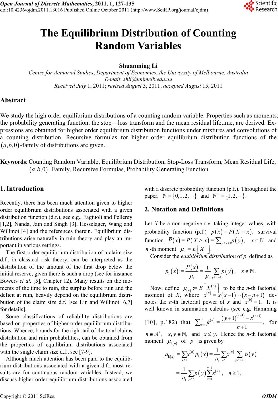
 Open Journal of Discrete Mathematics, 2011, 1, 127-135 doi:10.4236/ojdm.2011.13016 Published Online October 2011 (http://www.SciRP.org/journal/ojdm) Copyright © 2011 SciRes. OJDM The Equilibrium Distribution of Counting Random Variables Shuanming Li Centre for Actuarial Studies, Department of Economics, the University of Melbourne, Australia E-mail: shli@unimelb.edu.au Received July 1, 2011; revised August 3, 2011; accepted August 15, 2011 Abstract We study the high order equilibrium distributions of a counting random variable. Properties such as moments, the probability generating function, the stop—loss transform and the mean residual lifetime, are derived. Ex- pressions are obtained for higher order equilibrium distribution functions under mixtures and convolutions of a counting distribution. Recursive formulas for higher order equilibrium distribution functions of the -family of distributions are given. ,,0ab Keywords: Counting Random Variable, Equilibrium Distribution, Stop-Loss Transform, Mean Residual Life, Family, Recursive Formulas, Probability Generating Function ,,0ab 1. Introduction Recently, there has been much attention given to higher order equilibrium distributions associated with a given distribution function (d.f.), see e.g., Fagiuoli and Pellerey [1,2], Nanda, Jain and Singh [3], Hesselager, Wang and Willmot [4] and the references therein. Equilibrium dis- tributions arise naturally in ruin theory and play an im- portant in various settings. The first order equilibrium distribution of a claim size d.f., in classical risk theory, can be interpreted as the distribution of the amount of the first drop below the initial reserve, given there is such a drop (see for instance Bowers et al. [5], Chapter 12). Many results on the mo- ments of the time to ruin, the surplus before ruin and the deficit at ruin, heavily depend on the equilibrium distri- bution of the claim size d.f. [see Lin and Willmot [6,7] for details]. Some classifications of reliability distributions are based on properties of higher order equilibrium distribu- tions. Whence, bounds for the right tail of the total claims distribution and ruin probabilities, can be obtained from the properties of equilibrium distributions associated with the single claim size d.f., see [7-9]. Although much attention has been paid to the equilib- rium distributions associated with a given d.f., most re- sults are for continuous random variables. Instead, we discuss higher order equilibrium distributions associated with a discrete probability function (p.f.). Throughout the paper, =0,1,2, and =1,2, . 2. Notation and Definitions Let X be a non-negative r.v. taking integer values, with probability function (p.f.) survival function ==pxPX x, 1 = , yx =>xPXx py x and -th moment n=. n nEX Consider the equilibrium distribution of p, defined as 1 1 11 1 := =,. yx Px pxpy x Now, define := n nEX n xx to be the n-th factorial moment of X, where de- notes the n-th factorial power of x and It is well known in summation calculus (see e.g. Hamming =1x xn 0=1.x 1 [10], p.182) that 11 = 1 =, 1 nn yn kx yx kn for ,n ,xy , and . y Hence the n-th factorial moment 1: n of is given by 1 p 1 1: 11 1 1 2=1 1 1 == 1 =,1, nn nxxy yn yx 1x pxx py py xn 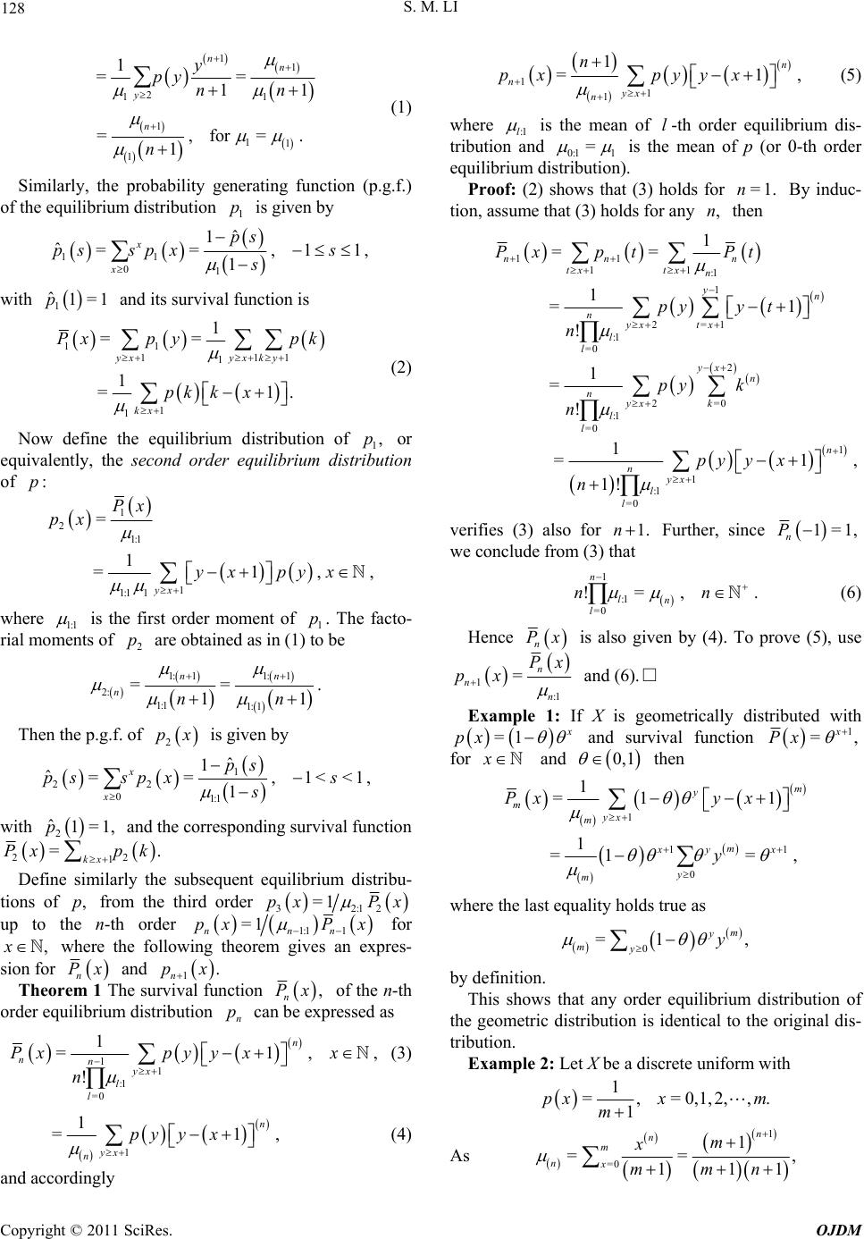 128 S. M. LI 11 2 1 1 11 1 1 == 11 =,for=. 1 nn y n y py nn n 1 (1) Similarly, the probability generating function (p.g.f.) of the equilibrium distribution is given by 1 p 11 01 ˆ 1 ˆ==,1 1 x x ps ps spxs s 1, with and its survival function is 1 ˆ1=1p 11 11 1 1 1 1 == 1 =1. yxyx ky kx Pxp ypk pk kx 1 (2) Now define the equilibrium distribution of 1 or equivalently, the second order equilibrium distribution of ,p :p 1 2 1:1 1 1:1 1 = 1 =1,, yx Px px yx pyx where 1:1 is the first order moment of 1. The facto- rial moments of are obtained as in (1) to be p 2 p 1: 11: 1 2: 1:1 1: 1 == 11 nn nnn . Then the p.g.f. of is given by 2 px 1 22 01:1 ˆ 1 ˆ==,1< 1 x x ps ps spxs s <1, with and the corresponding survival function 2 ˆ1=1,p 22 1 =. kx Px pk Define similarly the subsequent equilibrium distribu- tions of from the third order ,p 32:12 =1px Px up to the n-th order 1:1 1 =1 nnn pxP x for where the following theorem gives an expres- sion for ,x n Px and 1. n px Theorem 1 The survival function , n Px of the n-th order equilibrium distribution can be expressed as n p 1 1 :1 =0 1 =1 ! n nnyx l l Pxpy yxx n ,, (3) 1 1 =1, n yx n py yx (4) 1 1 1 1 =1 n nyx n n px pyyx , (5) where :1l is the mean of -th order equilibrium dis-l tribution and 0:1 1 = is the mean of p (or 0-th order equilibrium distribution). Proof: (2) shows that (3) holds for =1.n By induc- tion, assume that (3) holds for any ,n then and accordingly 11 11 :1 1 2=1 :1 =0 2 2=0 :1 =0 1 1 :1 =0 1 1 =1 ! 1 = ! 1 =1, 1! nn n txtx n yn nyx tx l l yx n nyx k l l n nyx l l py y t n py k n py yx n verifies (3) also for ==Px ptPt 1.n Further, since 1=1, n P we conclude from (3) th 1n n at :1 =0 !=, ln l n . (6) Hence n Px is also given by (4). To prove (5), use 1 :1 = and (6).□ n nn Px px Example 1: Ifetrically distributed with X is geom =1 px and survival function 1 =, x Px for x and 0,1 then 1 11 0 11 1 =1=, m myx m m xy x y m Py x y where the last equality holds true as , by definition. that any order equilibrium distribution of =1 y x =1 y my 0 m y This shows the geometric distribution is identical to the original dis- tribution. Example 2: Let X be a discrete uniform with 1 =,px 1m =0,1,2,, . m 1 =0 1 == 11 n n m nx m x mmn A s , 1 C opyright © 2011 SciRes. OJDM 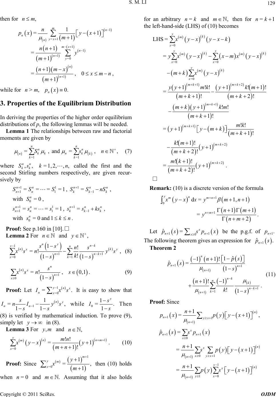 S. M. LI 129 then for ,nm 1 =1 1 1 1=0 1 1 =1 1 1 = 1 1 =,0, 1 mn nyx n mx n ny n n n pxy x m nn y m nmx mn m while for 3. Properties of the Equilibrium Distribution Lemma 1 The relationships between raw and factorial >,nm 0. n px In deriving the properties of the higher order equilibrium distributions of p, the following lemmas will be needed. moments are given by nn =1 =,and= ,, =1k nn kk n k nk k Ssn (7) where called the first and the secondectively, are given sively by ,, nn kk Ss Stirlin =1,2,, ,kn g numbers resprecur- 111 11 1 ====1, =, with nn n nnkk k n SSS SSnS 0 11 1 11 1 0 = 0 , ====1, =, with=0and1. nn nnnn n nnkk k n S ss s ssks skn Proof: See p.160 in [10] Lemma 2 For and .□ n,y 11 =! ny yn n 1 =0 = 1 1 !, ! 11 nk k y k ns nn xk ss sn ys k ss (8) 1 0 =!, 0,1. 1 n nx n x s xs ns s Proof: Let . (9) 1 =0 = yn nx xs It is easy to show that 1 1 1 =, 1 n nn s nI ys s while s 01 1 =. y I Then (8) is verified by mathematical induction. To prove (9), simply let in (8). Lemma 3 For and y ,ym ,n 1 1 . 1! yx y (10) Proof: Since =0xmn !! = ynnm mmn x 1 =0 1 = 1 m ym x y xm , then ( when and Assuming that it also holds for an arbitrary and then for 10) holds =0n.m =nk ,m=1nk th of (1mee left-hand-sides (LHS) 0) beco =0 LH = ym x yy k mm xy yxk yx yxxmx =0 =0 12 1 S = 1!!1!1! =1! 2! 1!! 1! !! =11! k k xx k m mk mk x yx mk yx yymk ykm mk km mk yymk mk =0 1 y x mk mk x mk mky mk 2 2 !1 =1. mk mk km y mk y mk □ Remark: (10) rete version of the formula !1 2! !1! 2! mk is a disc 1 0 111 =. 2 nm nm ynm d=1, 1 yn mmn xyx xymn Let 11 0 ˆ=x nn x ps spx be the p.g.f. of 1. n p The folloxpression for wing theorem gives an e 1.ps ˆn Theorem 2 11 1 ˆ 1 ! ˆ= 1 nn n ps ps s 1 =1 1 11 1! 1 . !1 n nk nk nk k n n n ks (11) Proof: Since 11 1 1 =1 n nyx n n px pyyx , 11 0 01 1 1 1=0 1 ˆ= 1 =1 1 =1 x nn x n x xyx n yn x yx n ps spx nspyyx npysyx Copyright © 2011 SciRes. OJDM  130 S. M. LI 1 1 1=0 1 1 1 1 1 1 1 1 =1 1 1 1 = 1 11 =1! 1 1! 1 ,by Lemma 2, !1 ˆ 1 11! = 1 yn yx yx n yy n y n y n nk y k n nk k n n n npyssx s npys ns s ny ks s ps n s 1 =1 1 1!1 . !1 nk nk nk k n n ks □ Theorem 3 : !! =,, ! nm nm n nm mn mn , (12) : =1 ! ! =, ! m mk nm nk k n ks nmn nk ,, (13) hwere :nm is . the -th moment of the distribution Proof: m n p :( ) 0 11 1=0 1 = =1 =! !! =. ! m nm n x yn m yx n y n nm n xpx npyxyx nm nm mn To prove (13), use as stated in Lemma 1, and (12) Consider now the stop-loss transform !1 ! ,by Lemma 3, nm mn npyy :: =1 =, mm nmk nk ks .□ π= EX x of the r.v. X (where the notation =>0aaIa ). For n p-loss tra nd by . Theorem and denote by h stonX (with p) a its n-th fac- formma 1 show ,x sform of n x d Lem n EX x the n-t probability function torial stop-loss trans tha EX 1 an t nx= n n EX xP 1 and P x =1 kk k k =EX x1. Let nn s n m ity function al st be a ra to b factori ndom variable following the probabil- Define n mx e the n-th op-loss transform of m p and n m EX x . m p EX to be the n-th stop-loss transformmhe following theorem holds. Th of T eorem 4 For .p n and, ,mx =! !! =1 ! n nm m Exmn mn Px mn (14) !! , nm m m nm EXx mn X =1 =1 ! ! =! mk k m EX x E mk ! ! =1 ! n n k m n nkmk mk k m ks mX x ks mPx mk n (15) Proof: The argument is similar to that in the above proof. Now define □ =>,,x mmm rx EXxXx ,m to be the mean residual lifetime (MR and L) of , m p = =m mm PX x hx PXx to be the hazard function of Then the following result holds. rate . m p Theorem 5 For x and ,m 11 mm Px mPx =1 1 mm m rx (16 ) 1 1 =. m xrx m h (17) Proof: 1 11 1 11 =>= 1 = 1 =1 =1,by (14). 1 m kx mmm mm kx kx m m mm m m kxpk rx EXxXx k xpkpk EX x Px Px mPx while m Px m Px 11 1 1 == 1 11 ==,by (16). 1 m mm mm m mm m m m px hx Px px Px px mrx Px Px This proves the conclusion.□ C opyright © 2011 SciRes. OJDM 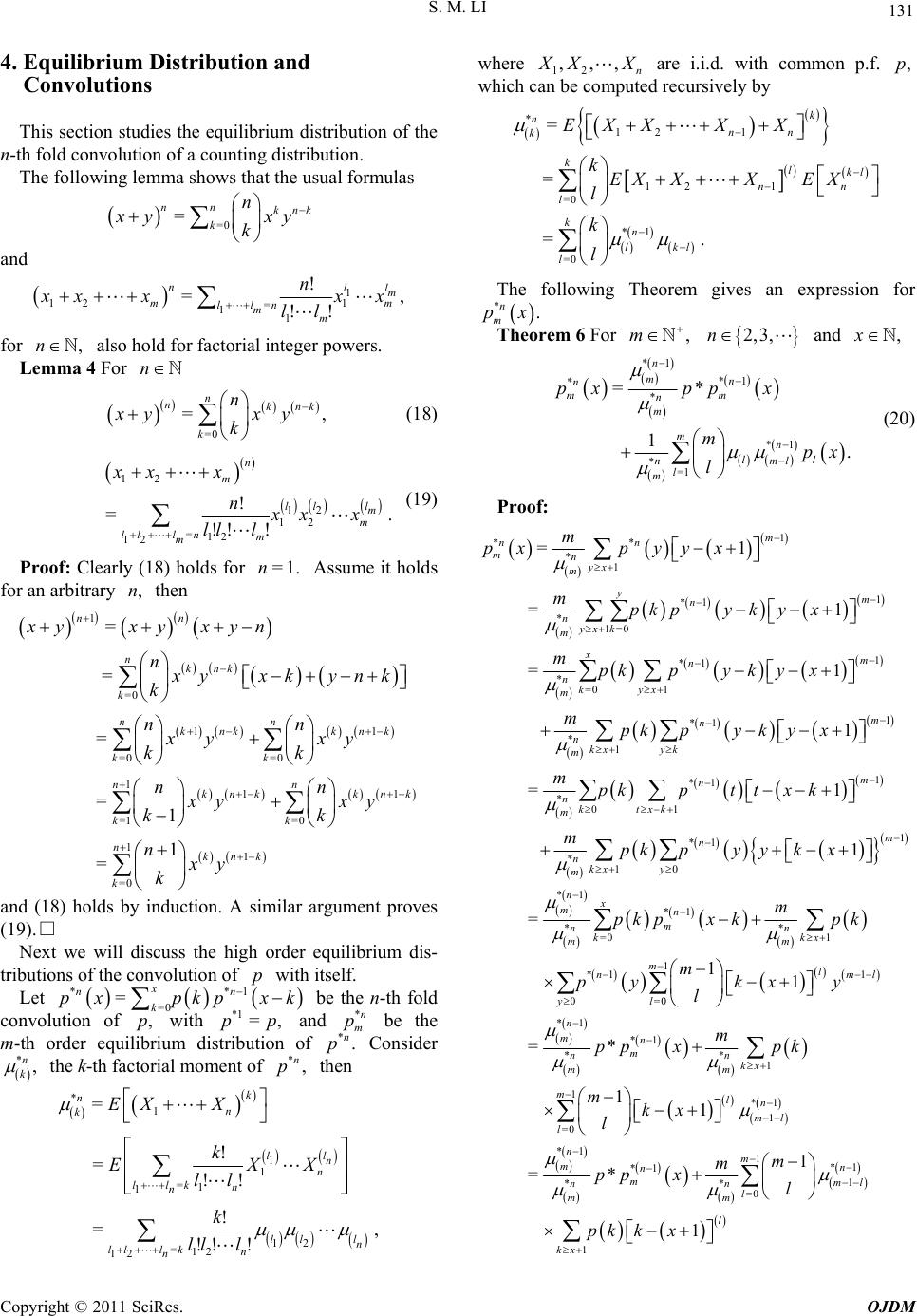 S. M. LI 131 4. Equilibrium Distribution and Convolutions section studies the equilibrium distribution of te n-th fold convolution of a counting distribution. The following lemma shows that the usual formulas This h =0 = nnknk k n yx k y and 1 12 ! nl l m n 1 = 11 = !! m ll n mm , m xxxx ll (18) for ,n also hold for factorial integer powers. Lemma 4 For n =0 =, n nknk k n xy xy k 12 12 12 =12 12 ll l nm m lds for =1.n Assume it ! =. !! ! n m l ll m m xx x nxxx lll (19) (18) h holds fo then and (18) holds by induction. A similar argument proves (19) Next we will discuss the high order equilibrium d- tributions of the convolution of with itself. Let 1 be the n-th fold convo and be the m-th onsider Proof: Clearly o r an arbitrary ,n 1 =0 11 =0 =0 11 =1 =0 11 =0 = = = 1 1 = nn nknk k nn knk knk kk n knk knk kk nknk k xyxyxyn nxyxk ynk k nn xy xy kk y xy kk nxy k 1 = n nn x .□ is p ** =0 =x nn k pxpkp xk lution of ,p with *1 =,pp order equilibrium distribution of *n m p *. n Cp *, n k the k-th factorial moment of *, n p then 12 =12 12 =, !!! lln ll l kn n k ll l e 12 ,,, n 1 ! l wher * 1 =k nn kEX X 1 1 =1 ! =!! l ln n ll kn n k EX X ll XX are i.i.d. wiommonth c p.f. whicrecursively by ,p h can be computed * 12 1 12 1 =0 *1 =0 = = =. k nnn k klkl nn l kn kl l l EXXX X kEX XXEX l k l The following Theorem gives an expression for *n. m px Theorem 6 ,m 2,3,n and ,x For *1 *1 * * *1 * =1 =* 1 . n mn n mm n m mnl lml nl m pxpp x mpx l (20) Proof: 1 ** * 1 1 *1 * 1=0 1 *1 * =0 1 1 *1 * 1 * 0 = n mn m xp 1 =1 =1 1 = m n yx m ym n nyxk m xm n nkyx m m n nkxyk m nktx m pyyx mpk pykyx mpkpykyx mpkpykyx mpk 1 *1 1 1 *1 * 10 *1 *1 ** =0 1 1 *1 1 0=0 *1 * 1 1 = 1 1 = m n k m n nkx y m nx mn m nn kkx mm ml nml yl n m m pttxk mpkpy ykx m pk pxkpk m pykx y l *1 * 1 1*1 1 =0 *1 1*1 *1 1 ** =0 1 * 1 1 1 =* 1 n m nn kx m mln ml l nm mn n mml nn l mm l kx m pp xpk mkx l m m pp xl pk kx Copyright © 2011 SciRes. OJDM 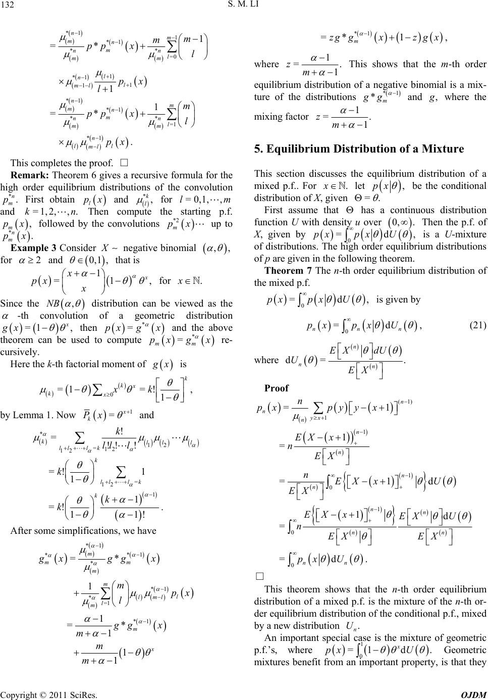 132 S. M. LI *1 1 *1 ** =0 1 *1 1 1 *1 *1 ** =1 *1 1 =* 1 1 =* . nm mn m nn l mm l nl ml nm mn m nn l mm nl lml m m pp xl px l m pp xl px This completes the proof. Remark: Theorem 6 gives a recursive formula for the high order equilibrium distributions of the convolution First obtain □ *. n m p l px and *, k l for om =0,1,,lm starting p.f. and =1,2, ,kn. Then cpute the , followed . xample 3 Con m px *n m px E by the co sider nvols ution *2 m px up to negative binomial ,, for 2 and at is , 1, th 1 0, =1 x px x for .x Since the ,NB distribution can be viewed as the -th cof a geometric distribution onvolution , =1 gx th can be used en and the above * =pxg x to compute theorem * = mm g x px re Here the k-th factorial moment of - cursively. x is 0 =1= !, 1 k kx kxxk by Lemma 1. Now 1 = k Px and * 12 =12 12 = 12 1 ! =!! ! =!1 1 1 =!. 11! kll l lll k k lll k k k ll l k k k After some simplifications, we have 1 1 x m *1 *1 * 1 m g x x m m *=* m gx g * 1 * =1 *1 1 1 =* mm m m l lml l m mp l gg x *1 =*1, m zg gxx z g where 1 =. 1 zm This shows that the m-th order ution onomial is a mix- ture of the distributions *1 *m gg equilibrium distribf a negative bi and , where the mixing factor 1 =. 1 zm 5. Equilibrium Distribut i o n o f a M i x t ure ses the equil distribution of a This section discusibrium mixed p.f.. For let ,px .x be the conditional distribution of X, given =. First assume that has a continuous distribution function U with dens over Then the p.f. of X, given by ity u 0, . U 0 =d,px px equilibriu igh is a Uixture of distributions. The h order m distributions of p are given in the following theorem. Theorem 7 The n-th order equilibrium distribution of the mixed p.f. -m =d,pxpx U 0 is given by 0 =d nnn pxpx U, (21) where d= n nn EX dU UEX . Proof =d. nn px U (1) 1 1 1 0 0 =1 1 = 1d n nyx n n n nn nn n pxpyy x EX x nEX n X xEX U EX EX 1n 0 =1d nEX x U EX = E n shows n-th . is the mixture of the n-th or- de ant i □ This theorem that the order equilibrium distribution of a mixed p.f r equilibrium distribution of the conditional p.f., mixed by a new distribution . n U An importxture of geometric p.f.’s, where 1 0 =1d . x px U special case is the m Geometric mixtures benefit from an important property, is that they C opyright © 2011 SciRes. OJDM 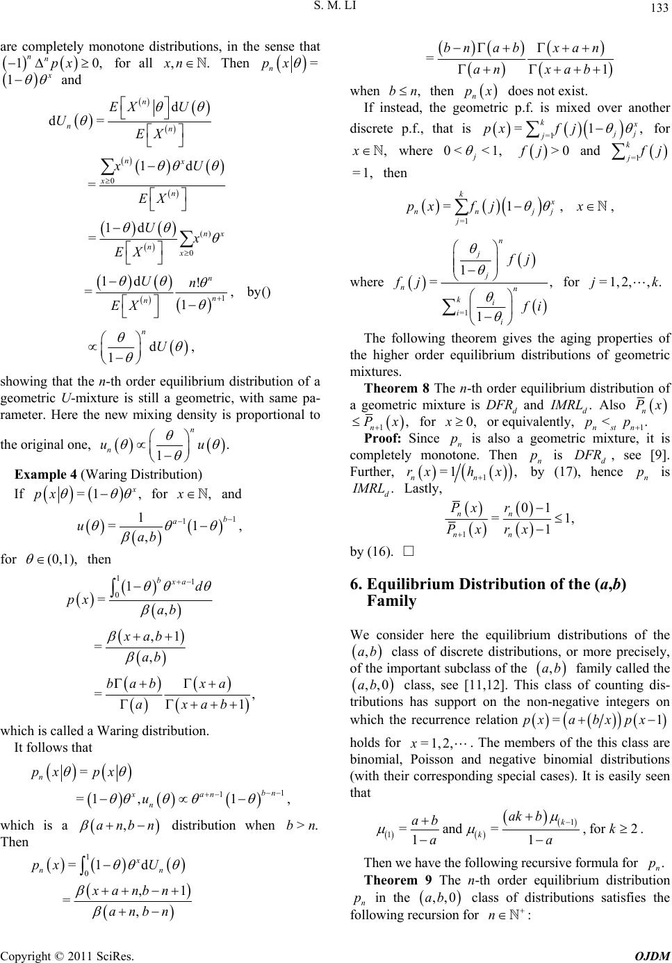 S. M. LI 133 ar 0, for all Then e completely monotone distributions, in the sense that 1 nnpx , .xn = n px 1 and () 0 d 1d 0 1 d= = 1d = 1d ! =,by() 1 d, 1 n nn nx x n nx nx n n n n EX U UEX xU EX Ux EX Un EX U at the n-th order equilibrium distribution of a U-mixture is still a geometric, with same pa- ter. Here the new mixing density is proportional to al one, showing th geometric rame the origin . 1 n n uu Example 4 (Waring Distribution) If =1, px for ,x and 1 1 1 =1, , b a u ab for (0, 1), then 11 01 =, bxa d px ab ,1 =, =, 1 xab ab bab xa axab Waring distribution. which is called a It follows that 1 1 = n px which is a Then =1,1, bn xa n n px u distribution when ,anbn >.bn 1 0 =1 d ,1 px =1 bn abxan an xab when ,bn then does not exist. n px If instead, the geometric p.f. is mixed over another discrete p.f., that , is =1 =1 k j f j j px for =, x nn U xanbn anbn ,x 1, where 0< < j 0f and >j =1 k j j =1 , then , where =1, kx nnjj pxfjx =1 j =1 1 =, 1 n j j nn ki ii fj fj i for =1,2,, .jk The following theorem gives the aging properties of the higher order equilibrium distributions of geometric mixtures. um distribution of Theorem 8 The n-th order equilibri a gure is DFR and eometric mixtd. d MRL Also n Px ,Px for 1n equivalently, 0,x or 1 <. nstn pp ixture, it is Proof: Sincege completely monotone. Then is see [9]. Further, p nis also a ometric m n pd DFR , 1 =1 , nn rxh x by (1nce is 7), hen p . d MRL Lastly, 1 01 =1 1 nn nn Px r Px rx , by (16). 6. Equilibrium Distribution of the (a,b) Family nside tions of the □ We cor here the equilibrium distribu ,b class of discrete distributions, or more precisely, the important subclass of the ,ab famthe a of ily called ,,0ab class, see [11 dis- the non-negative integers h the re ,12]. Thounting tributions has support on on whiccurrence relation is class of c =1pxabx px holds for . The members of the this class are binomial, Poisson and negative binomial distributions (with their corresponding special cases). It is easily seen that =1 ,2,x 1 1=and= , k for2. 11 k ak b ab k aa Then we have the following recursive formula for . n p Theorem 9 The n-th order equilibrium distribution n p in the ,,0ab class of distributions satisfies the following recursion for n : Copyright © 2011 SciRes. OJDM 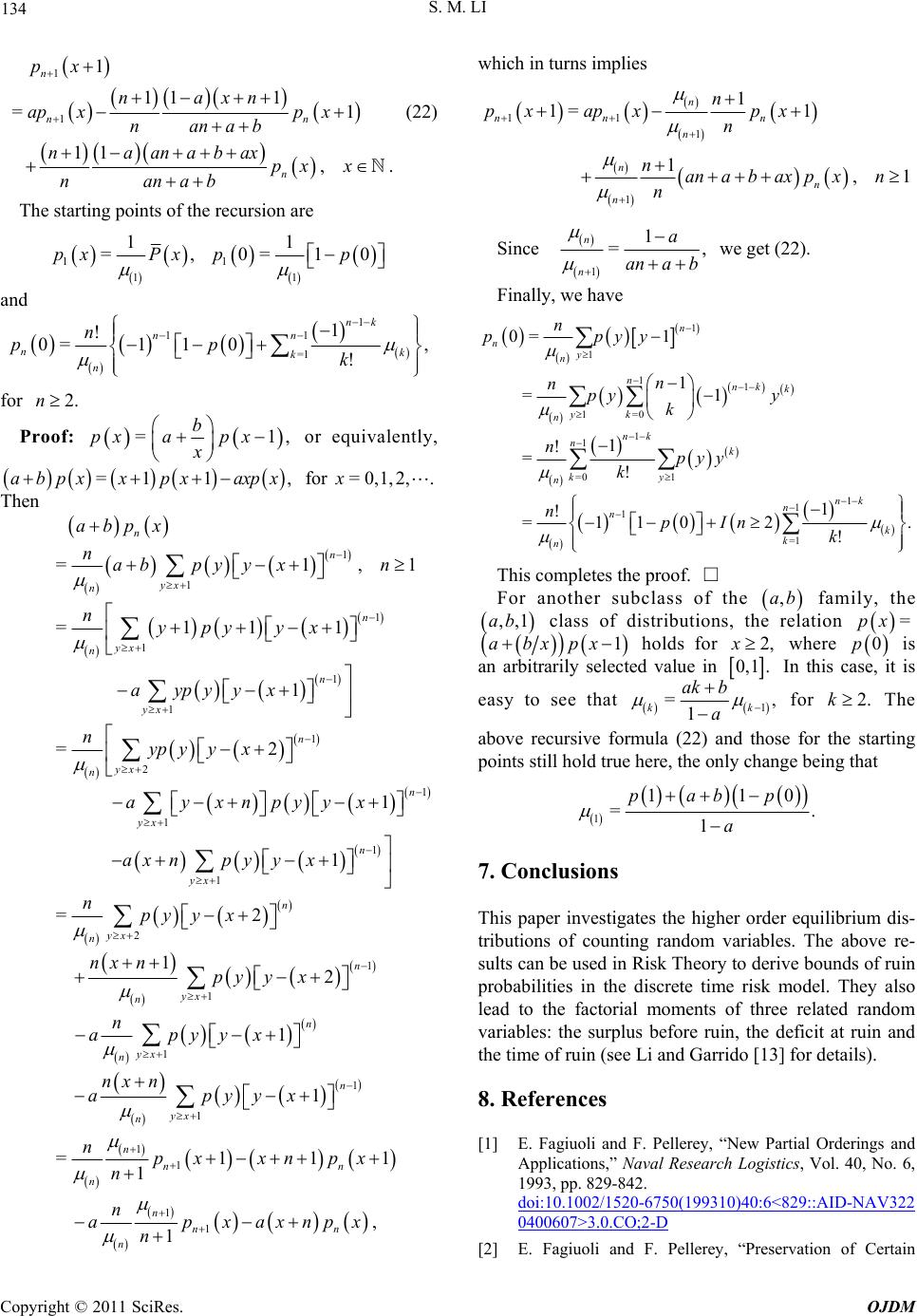 134 S. M. LI 11 ,. n nana b axpx x nanab The starting poinursion are 1 11 1 =1 n nn na xn ap xnanab 1 1 p x a (22) ts of the rec px 1 1 1 =,px Px 1 1 1 0= 1 0pp and 11 =1 0= 110! nn nk k n pp k 1 1 !, nk n r Pro fo 2.n of: =1, b pxapx x or equivalently, =1 1,x pxaxpx for =0,1,2, .x Then abpx 1 =2 n n yp y yx ay n 1 n n 1 1 1 2 1 1 1 1 yx n n yx yx yx yx ab ay pyyx xpyyx ax n 1 1 1 =1 ,1 =111 n yx n n py yxn nypy yx abpx n n 1 2 1 1 1 1 1 1 1 1 1 1 =2 2 1 1 =111 1 , 1 n n yx n n yx n n yx n n yx n n nn n n nn n py yx npyyx n apyyx nx n apyyx npxxnpx n n apxaxnpx n in turns implies 1 nxnpy yx which 11 1 1 1 1= 1 1 ,1 n nnn n n n n n px apxpx n nan ab axpxn n 1 1 =, n n a an a b Since we get (22). Finally, we have 1 1 11 1=0 1 1 =0 1 1 1 1 =1 0= 1 1 =1 1 ! =! 1 ! =1102. ! n ny n nnk k yk n nk nk ky n nk n n k k n n ppyy n npy y k npyy k npIn k This completes the proof. For another subclass of the family, the □ ,ab ,,1ab class of distributions, ttion he rela =px 1abxpx holds forere x2, wh 0p is an arbitrarily selected value in 0,1. In this easy to see that case, it is 1 =, 1 kk ak b a for The above recursive formula (22) and those for the starting points still hold true here, the only change being that 2.k 1 11 =. 1 pabp a 0 7. Conclusions This paper investigates the higher order equilibrium dis- tributions of counting random variables. The above re- sults can be used in Risk Theory to derive bounds of ruin probabilities in the discrete time risk model. They also leade factorial momentated random va the surplus before t at ruin and the ti Garrido [13] for details). 8. References [1] E. Fagiuoli and F. Pellerey, “New Partial Orderings and Applications,” Naval Research Logistics, Vol. 40, No. 6, 1993, pp. 829-842. to ths of three rel riables:ruin, the defici me of ruin (see Li and doi:10.1002/1520-6750(199310)40:6<829::AID-NAV322 0400607>3.0.CO;2-D [2] E. Fagiuoli and F. Pellerey, “Preservation of Certain C opyright © 2011 SciRes. OJDM 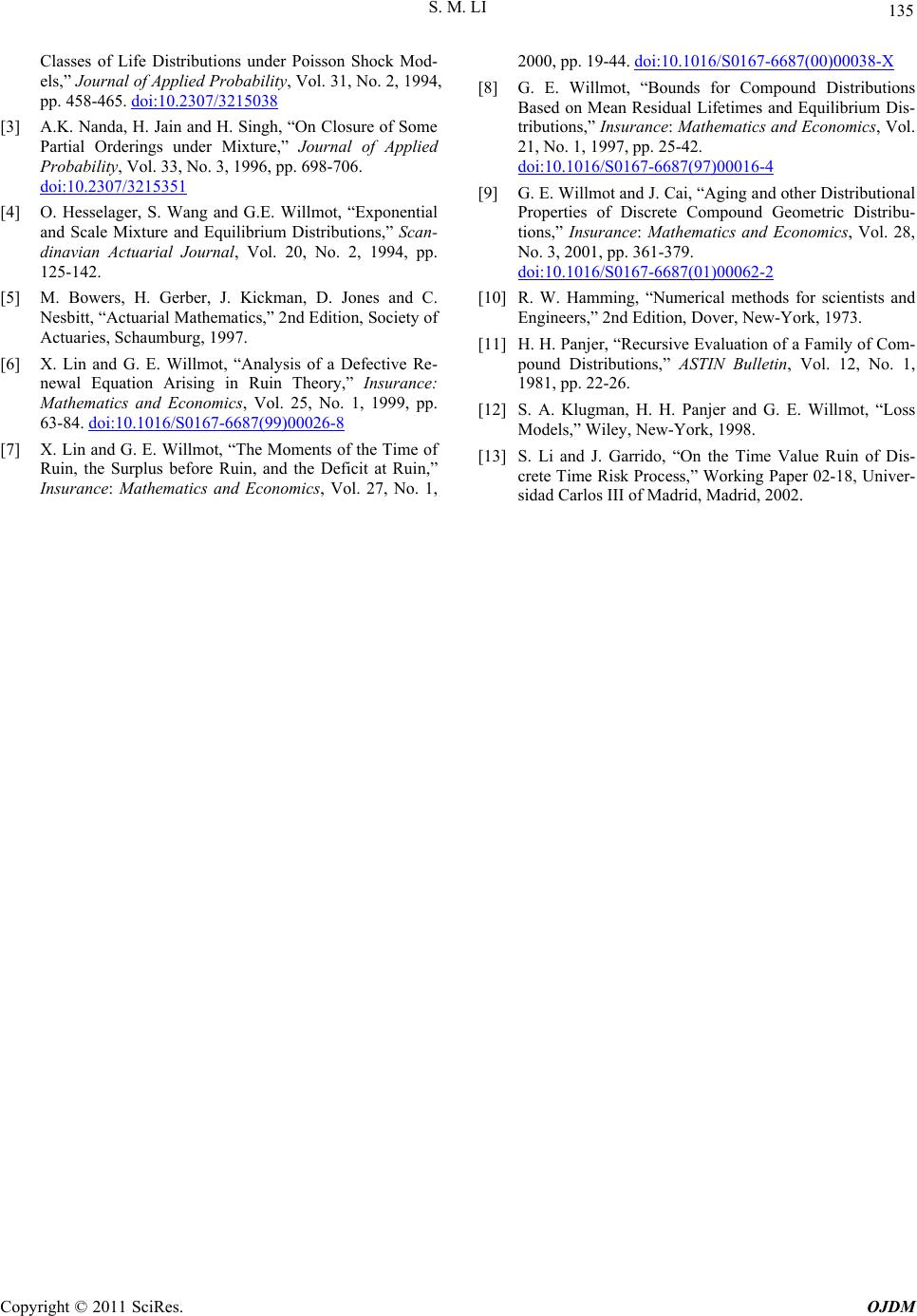 S. M. LI Copyright © 2011 SciRes. OJDM 135 Classes of Life Distributions under Poisson Shock Mod- els,” Journal of Applied Probability, Vol. 31, No. 2, 1994, pp. 458-465. doi:10.2307/3215038 [3] A.K. Nanda, H. Jain and H. Singh, “On Closure of Some Partial Orderings under Mixture,” Journal of Applied Probability, Vol. 33, No. 3, 1996, pp. 698-706. doi:10.2307/3215351 [4] O. Hesselager, S. Wang and G.E. Willmot, “Exponential and Scale Mixture and Equilibrium Distributions,” Scan- dinavian Actuarial Journal, Vol. 20, No. 2, 1994, pp. 125-142. [5] Kickman, D. Jones and C. atics,” 2nd Edition, Socie [6] X. Lin ve Re newal Equationuin T Vol. M. Bowers, H. Gerber, J. Nesbitt, “Actuarial Mathem ty of Actuaries, Schaumburg, 1997. and G. E. Willmot, “Analysis of a Defecti- Arising in Rheory,” Insurance: Mathematics and Economics, 25, No. 1, 1999, pp. 63-84. doi:10.1016/S0167-6687(99)00026-8 [7] X. Lin and G. E.ents ofime of Willmot, “The Mom the T Ruin, the Surplus before Ruin, and the Deficit at Ruin,” Insurance: Mathematics and Economics, Vol. 27, No. 1, 2000, pp. 19-44. doi:10.1016/S0167-6687(00)00038-X [8] G. E. Willmot, “Bounds for Compound Distributions Based on Mean Residual Lifetimes and Equilibrium Dis- tributions,” Insurance: Mathematics and Economics, Vol. 21, No. 1, 1997, pp. 25-42. doi:10.1016/S0167-6687(97)00016-4 [9] G. E. Willmot and J. Cai, “Aging and other Dist Properties of Discrete ributional Compound Geometric Distribu- tions,” Insurance: Mathematics and Economics, Vol. 28, No. 3, 2001, pp. 361-379. doi:10.1016/S0167-6687(01)00062-2 [10] R. W. Hamming, “Numerical methods for scientists and Bulletin, Vol. 12, No. 1, Engineers,” 2nd Edition, Dover, New-York, 1973. [11] H. H. Panjer, “Recursive Evaluation of a Family of Com- pound Distributions,” ASTIN 1981, pp. 22-26. [12] S. A. Klugman, H. H. Panjer and G. E. Willmot, “Loss Models,” Wiley, New-York, 1998. [13] S. Li and J. Garrido, “On the Time Value Ruin of Dis- crete Time Risk Process,” Working Paper 02-18, Univer- sidad Carlos III of Madrid, Madrid, 2002.
|