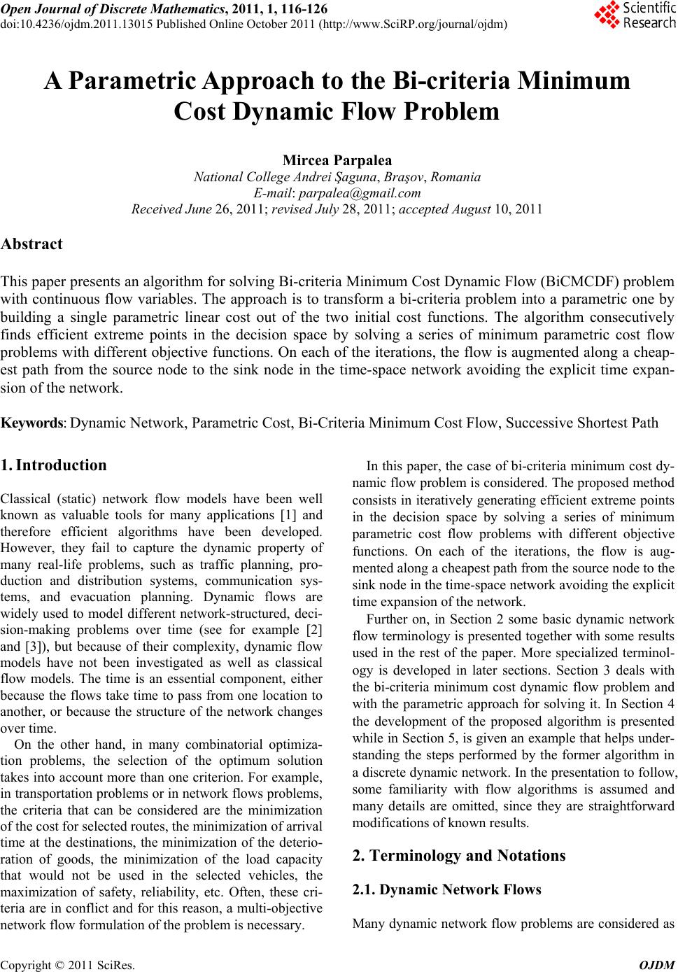Open Journal of Discrete Mathematics, 2011, 1, 116-126
doi:10.4236/ojdm.2011.13015 Published Online October 2011 (http://www.SciRP.org/journal/ojdm)
A Parametric Approach to the Bi-criteria Minimum
Cost Dynamic Flow Problem
Mircea Parpalea
National College Andrei Şaguna, Braşov, Romania
Received June 26, 2011; revised July 28, 2011; accepted August 10, 2011
Abstract
This paper presents an algorithm for solving Bi-criteria Minimum Cost Dynamic Flow (BiCMCDF) problem
with continuous flow variables. The approach is to transform a bi-criteria problem into a parametric one by
building a single parametric linear cost out of the two initial cost functions. The algorithm consecutively
finds efficient extreme points in the decision space by solving a series of minimum parametric cost flow
problems with different objective functions. On each of the iterations, the flow is augmented along a cheap-
est path from the source node to the sink node in the time-space network avoiding the explicit time expan-
sion of the network.
Keywords: Dynamic Network, Parametric Cost, Bi-Criteria Minimum Cost Flow, Successive Shortest Path
1. Introduction
Classical (static) network flow models have been well
known as valuable tools for many applications [1] and
therefore efficient algorithms have been developed.
However, they fail to capture the dynamic property of
many real-life problems, such as traffic planning, pro-
duction and distribution systems, communication sys-
tems, and evacuation planning. Dynamic flows are
widely used to model different network-structured, deci-
sion-making problems over time (see for example [2]
and [3]), but because of their complexity, dynamic flow
models have not been investigated as well as classical
flow models. The time is an essential component, either
because the flows take time to pass from one location to
another, or because the structure of the network changes
over time.
On the other hand, in many combinatorial optimiza-
tion problems, the selection of the optimum solution
takes into account more than one criterion. For example,
in transportation problems or in network flows problems,
the criteria that can be considered are the minimization
of the cost for selected routes, the minimization of arrival
time at the destinations, the minimization of the deterio-
ration of goods, the minimization of the load capacity
that would not be used in the selected vehicles, the
maximization of safety, reliability, etc. Often, these cri-
teria are in conflict and for this reason, a multi-objective
network flow formulation of the problem is necessary.
In this paper, the case of bi-criteria minimum cost dy-
namic flow problem is considered. The proposed method
consists in iteratively generating efficient extreme points
in the decision space by solving a series of minimum
parametric cost flow problems with different objective
functions. On each of the iterations, the flow is aug-
mented along a cheapest path from the source node to the
sink node in the time-space network avoiding the explicit
time expansion of the network.
Further on, in Section 2 some basic dynamic network
flow terminology is presented together with some results
used in the rest of the paper. More specialized terminol-
ogy is developed in later sections. Section 3 deals with
the bi-criteria minimum cost dynamic flow problem and
with the parametric approach for solving it. In Section 4
the development of the proposed algorithm is presented
while in Section 5, is given an example that helps under-
standing the steps performed by the former algorithm in
a discrete dynamic network. In the presentation to follow,
some familiarity with flow algorithms is assumed and
many details are omitted, since they are straightforward
modifications of known results.
2. Terminology and Notations
2.1. Dynamic Network Flows
Many dynamic network flow problems are considered as

M. PARPALEA 117

extensions of static network flow problems. These in-
clude maximum dynamic flow and minimum cost dy-
namic flow problems. The maximum dynamic flow
problem seeks a dynamic flow which sends as many as
possible a commodity from a single source to a single
sink of the network within the time horizon T. The
minimum cost dynamic flow problem seeks a dynamic
flow that minimizes the total shipment cost of a com-
modity in order to satisfy demands at certain nodes
within T.
2.2. Discrete-Time Dynamic Network Flows
A discrete dynamic network is a directed
graph where is a set of nodes with

,,GNAT

,,Ni i
Nn, A is a set of arcs with

,,aa
A
m

,
and T is a finite time horizon discretized into the set

1, ,

0,
H
T

,ij
. An arc a from node i to node j is usu-
ally also denoted by . The following functions are
associated with each arc

,aijA

: the time-de-
pendent capacity (upper bound) function


,;uij

,
which represents the maximum
amount of flow that can enter the arc at time

:0,1,

,T uA

,ij


,
the time-dependent transit time function


,;hij

,
, and the time-dependent cost
function

:0,1,

,T

,;cij
hA

,


:0,1,,TcA   which
represents the cost for sending one unit of flow through
the arc


,ij at time

. Time is measured in discrete
steps, so that if one unit of flow leaves node i at time

on arc , one unit of flow arrives at node j at
time

,j

,;j
ai
hi

 , where


,;hij

is the transit time
on arc a. The time horizon T is the time until which the
flow can travel in the network. The demand-supply func-
tion vi 
;,

represents the de-
mand of node i at the time-moment ,
if vi or the supply of node i at the time-moment
, if . The network has two
special nodes: a source node s with for
and there exists at least one moment of
time 0 such that ; and a sink
node t with for and there
exists at least one moment of time 1 such
that . The condition required for the flow to

:0,1,vN
N
0
 
;vi  


1, ,T

;0vt  
0
vi

,T

0
vs

0
;vs  

0,1,,T  
0,1,
 

;0 

0,1,,T

;0  
0


,T


;
, ,T

, ,T
0,

1
; 

0,1  
0,1  

vt
exist it that

0,1,,TiN  



Definition 1: [4] A feasible dynamic flow


,;
f
ij

(feasible flow over time) on with
time horizon T is a function

,,hcT

,,T
,,,GN
Au
:0,1fA


that satisfies the following constraints:











,,
,; 0
,;,;,;; ,
jijAj jiA
hji
fijf jihjivi









;0,1,,iN T    (1.a)



 


0,;,;,0,1,,,, ;
f
ijuijTij A 

 
(1.b)
 
,;0, ,,,;1,
f
ijijAT hijT     (1.c)
where


,;
f
ij

determines the rate of flow (per time
unit) entering arc


,ij at time

.
Capacity constraints (1.b) mean that in a feasible dy-
namic flow, at most


,;uij

units of flow can enter
the arc


,ij at the time-moment

. It is easy to ob-
serve that the flow does not enter arc at time

,ij


if it has to leave the arc after time T; this is ensured by
condition (1.c). The total cost of the dynamic flow


,;
f
ij

in a discrete-time dynamic network is defined
as:



0,1,,,
,; ,;
TijA
Cffij cij









(2)
2.3. Time-Space Network
In the discrete time model, a useful tool for studying the
minimum cost flow over time problem is the time-space
network. The time-space network is a static network
constructed by expanding the original network in the
time dimension by considering a separate copy of every
node iN

at every discrete time step in the time hori-
zon T,


0,1, ,T  .
A node-time pair (NTP)

,i

refers to a particular
node iN

at a particular time step , i.e.,

0,1,,T  




0,1,T  ,iN ,.
The NTP


,i1

is said to be linked to the NTP


2
,j

if either
i)


ij,A

and

21 1
,;hi j

  , or
ii)


,ji A

and

,;hji
12 2

  .
Definition 2: [5] The time-space network of the
original dynamic network G is defined as follows:
T
G



:,|,0,1,,
T
NiiN T  ; (3.a)
 








:,,,,;
0,;, ,;
T
Aa ijhij
T hijijA

 

 

 (3.b)




:;for
TT
uauaa A

 ;

 (3.c)




:;for
TT
cacaaA

 .

 (3.d)

For every arc


,ij A

with traversal time


,;hij

,
capacity


,;uij

and cost


,;cij

, the time-space
network contains arcs
T
G

,,ij
  

,;hij,

 
for


0,1,,, ;Thij

  with capacities


,;uij

and costs


,;jci

.

M. PARPALEA
118
flow For the

;fa


in the dynamic network G, the
function

T
fa

that re
e
presents the corresponding flow
in the timnetwork T G is defined as:
 
;, .
TT
fa faA

 
e-spac
a (4)
A (discrete-time) dynamic path
qu
is defined as a se-
ence of distinct, consecutively linked NTPs:



 
,:,,, ,,,Pi iiiii


112 2
121 1
22
,
,.
qq
kkk kkk
i

  
  (5)
.4. Time-Dependent Residual Network
he time-dependent residual network corresponding to a
2
T
feasible flow f can be viewed as the static residual net-
work of the time-space network corresponding to the
dynamic network.
For

,;
f
ij

being the flow entering arc


,ij at
time

, an additional flow

,; ,uijf ij;

 de-
partinfrom node i at time g

to arc node j along the


,ij can be sent. Also,


,;
f
ij

units of flow can be
from node j depart

,;hij sent ing at time

  and
consequently arriving at node i at time

ov
xistin
er the arc

,ij, which amounts to cancelling the eg flow on
c. Here, an arc with negative travel time (i.e. de-
parting at

,;hij
the ar

  and arriving at

) is consid-
ered. Where unit of flow from i at time as sending a

to j along

,ij increases the flow cost by


,;cij

units, sendingunit of flow in reverse direction fr
departing at time

,;hij
a om j

  to i on the same arc de-
creases the flow cost by


,j;ci

units.
Considering the aboved idease mention, the residual
ne
5] The residual dynamic network with
re
twork with respect to a current dynamic flow f is de-
fined as follows.
Definition 3: [
spect to a given feasible dynamic flow f is defined as
  
:, ,GfNAf T with
 


:
A
fAfAf


where
  


:, ,,,;
with, ;, ;0

fij ijAThij
uijf ij
A




 (6.a)

  


:, ,,,;
with,;0
AfijjiAThji
fji




 (6.b)
While the direct arcs have the same
tra
 
,ijA f


nsit times

,;hij

a

,;jnd costs ci


as in the
original dynamrk G, the artificial reverse arcs
 
,ijA f

 in the residual dynamic network
ic netwo


Gf
ith the following attributes:



,;,; :,;hijh jih ji
are provided w

,

   (7)



 
,;,;:,; ,cijh jic ji


  
with
(8)




,,0,; ,,;jiAh jiTfji 

0 

 
e residual capacities of the arcs

,ij in the
.
resid-Th
namic network ual dy


Gf are defiollowned as fs:




,;:,;,; ,rijuf ij
  
,, 0 ,;
ij
ij AhijT

  (9.a)
   



 
 
, ;,;,;,
,,0,;
rijh jifji
jiAh jiT




 

 (9.b)
Definition 4: [6] A dynamic path


i
12
,, ,
q
Psi ii


from dynamic augmenting
path if
node s to node i is said to be a


,; 0ri i  
1kk kkk
for and
 
1
,ii Afk

1, ,1q

.
Defin n a dyhe residual
f a
ition 5: [6] Givenamic flow f, t
capacity o dynamic augmenting path


12
,, ,
q
Psi iii


is defined by:

 
1
11
:min ,;
kk k
kq
rPri i,



 (10)
for




1
,
kk
ii Af
, 1, ,1kq

.
e cost of a dyDefinition 6: [6] Thnamic augmenting
path


,, ,
12 q
P
sii ii

 is defined by:




;1,,1
k
CPcifork q 

 
1
1
,
:,
kk
kk
ii Af

i




A dynamic augmenting path

12
,, ,
q
P
siii i
dynamic shortest augmenting path (DSAP)
is
referred to as a
from node 1
s
i

to node q ii if




'CP CP for
all dynamic augmenting paths 'P from node s to node i.
A dynamih c pat


 


11 22
,: ,
qqq
Pi ii
1
,,,,,i i

  is
ca yc e if lled a dynamic cl and
1q
ii1q

 
c cycle whose t
. A g
tiv dyotal co
than z
ow
Problem
Thminimum cost dynamic flow problem is
determine how a given amount of flow that simulta-
ne a-
e cycle is defined as ast nami
is negative and whose capacity is greaterero.
3. Bi-Criteria Minimum Cost Dynamic Fl
e bi-criteria
to
neously minimizes two total costs should be sent from a
source node to a sink node within the time horizon T,
subject to the capacity limits on the arcs of the network.
The successive shortest path approach adapted to the
dynamic residual network is based on solving a series of
successive shortest path problems, where each is solved
in a residual time-space network. An amount of flow
equal to the capacity of each minimum cost path ob-
tained is augmented, until the entire flow has been sent

M. PARPALEA 119
etwork with a node
t nd a finite time horizon T discretized
from the source to the sink. The main difference among
the algorithms consists in solving the shortest path prob-
lem in the dynamic residual network.
3.1. The Problem Formulation
Let

,,GNAT be a dynamic n
se N, an arc set A a
e set

0,1,
ink no
into th

,T. Without loss of generality, we
consider that no arcs are entering in the source node or
leaving the sConsidering the time-dependent
capacity (upper bound) function

de.

,; ,uij

:uA


0,1, ,T , the time-dependent transit time func-
tion

,; ,hij


:0,1,,hA T
tions

,; ,
k
cij
,  and the time-de-
pendent cost func



:0,1,,
k
cA T

,
repre the k-th objective
function, 1, 2k, for se
the arc
senting the cost associated with
nding one unit of flow through


,ij at time

, the BiCMCDF problem can be
stated as fie flow function

nding th

:0,1,,fA T


that satihe followig constraints:

minimize, ;
T
kk
yf cij
sfies tn

0(,)
, ;,
1, 2;
ij A
fij
k







 (11.a)
subject to:



0, ,;
,;
T
it Ahit
f
it v




  (11.b)





,,,;
,;
,
jijAj jiAhji
fij f
iN st
 



 

(11.c)

,
,; 0,ji  
 

0,;,;, 0,1,,
,.
f
ij uijT
ij A
 


(11.d)
The value of the dynamic flow for a time
denoted by v. Any vector f that satisfies the constraint
(1
horizon T is
1.b), the flow conservation constraint (11.c) at the dif-
ferent node-time pairs and the bound constraint (11.d) is
called a feasible solution of the bi-criteria minimum cost
dynamic flow (BiCMCDF) problem.
The set of feasible solutions or decision space is de-
noted by F and its image through
 


12
,YFyfyffF
is called objective space.
In general, there is no feasible solution
imultaneously minimizes both
ob
of the (Bi-
CMCDF) problem that s
jectives. In other words, an optimum global solution
does not exist. For this reason, the solutions of these
problems are searched for among the set of efficient
points.
Definition 7: [7] A feasible solution
f
F of the
bi-criteria minimum cost flow problem is cefficient
if,
alled
feasiband only if, there does not exist another le solu-
tion '
f
F

so that




'
kk
y
fyf for all k values
and




'
kk
y
fyf for at least one k.
De 8: [7] finition


f is a non-doYminated criterion
vector if
f
is an herwiseefficient solution. Ot


Yf
is
ed by
a dominated criterctor.
The set of efficient solutions of F will be denot
ion ve


EF while, by extension, EY


F is called the set
of non-dominated solutions of


YF. It is well known
characterize that to


EYF



 bi-criteria con-
tinuous minimum cost flow probt is only necessary
to identify the extreme points of

YF. The set
of efficient extreme points of F will be denoted by and
by
for the
lem, i
ent effici


ex
EF and the corresponding points of


F will
be denoted by
Y


ex
EYF



.
3.2. The Parametric Approach
g (BCLP) problems,
ass and Saaty [8] provide an algorithm using the para-
For the bi-criteria linear programmin
G
metric programming technique. Geoffrion [9] discusses
the availability of parametric programming for a broader
class of bi-criteria problems. The functions


1
y
f and


2
y
f are assumed to be convex and the feasible re-
gion F is a compact convex set. The parapro-
ing problem is defined as:
metric
gramm




12
minimize 1yfyfyf
fF
 

λλ
λsubject to,for01 (12)
He’s procedure is not radically different from
Gass and Saaty [8].
that of
Lemma 1: [9] If 0
f
is efficient, then there exists a
scalar 0
λ
in the unit interval such that 0
f
is an opti-
mrem
e
fo
al solution of the parametric programming problem.
Theo 1: [9] The set of all efficient extreme points
of the bi-criteria minimum cost flow problem can b
und by solving (12) for each
λ
in the unit interval.
Lemma 2: [9] For each fixed value of
λ
satisfying
0

λ1, the optimal solution(12) is a compact line of
segment in the objective space. If


1
y
f nd a


2
y
f
dpoints of the line segment, then

are the en

 
121
11ytf -tftyf-tyf  2
for all
,
,t 01t

.
Aneja and Nair [10] developed a simple algorithm for
riransporion problems. Their procedure gen-
er
bi-critea ttat
ates efficient extreme points on the objective space


YF rather than on the decision space. A series of
single objective problems are solved with different ob-
functions and each problems leads to either a new jective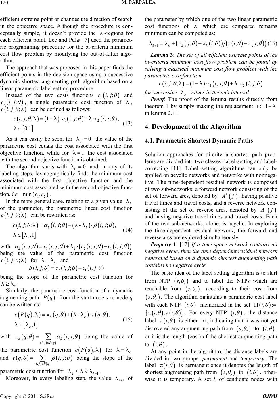

M. PARPALEA
120
efficient extreme point or changes the direction of search
in the objective space. Although the procedure is con-
ceptually simple, it doesn’t provide the
λ
-regions for
each efficient point. Lee and Pulat [7] used the paramet-
ric programming procedure for the bi-critia minimum
cost flow problem by modifying the out-of-kilter algo-
rithm.
The approach that was proposed in this paper finds the
efficien
er
t points in the decision space using a successive
dynamic shortest augmenting path algorithm based on a
linear parametric label setting procedure.
Instead of the two costs functions

1,;cij

and

2,;cij

, a single parametric cost function of
λ
,

,;;ij  c
λ
can be defined as follows:
 
12
;1,;,; ,c ijcij


,;
0, 1
cij

  λλ λ
λ (13)
As it can easily be seen, for talue
parametric cost equals the cowith the first
ob
mum cost
as
0
0
λ
st associate
1 th
he v
d
of the
jective function, while for λe cost associated
with the second objective function is obtained.
The algorithm starts with 0 and, in any of its
labeling steps, lexicographically finds the mini

0
λ
jectivesociated with the first ob function and the
minimum cost associated with the second objective func-
tion, i.e.

12
min ,cc .
In the more general case, relating to a given value k
λ
of the parameter, the parametric linear cost function

,;;ij  c
λ
can be rewritten as:


 
;,;,; ,
kk
ij ij

,;
,1
k
cij

  λλ-λ
λλ (14)
with










121
,; ,;,;
kk
ijc ijcijc i,;j

  λ
he value of the paramefunction

;; 

being ttric cost

,cij
λ
for k λ
λ
and

21
,;,; ,;ijcijc ij

 
slope parabeing the of themetric cost function for
k
λ
λ
.
Similarly, the parametric cost function of a dynamic
augmenting path from the start node s to node q
ca

Pq
n be written as:




 
,,,cPq qq

π,
,1
kk
k

 λλ-λ

λλ (15)
with

;j
 

,
π,,
kk
ij Pq
qi



 being te
rametric cost function
hvalue of
the pa


,Pq

c
λ
for k

λ
λ
and
 
,,qi

;j

,ij Pq

   being the slope

of the
of
of the two linear parametric
co
param 1kk λ
etric cost function for λ
λ
.
Moreover, in every lavalue beling step, the 1k

λ
the parameter by which one
st functions of
λ
which are compared ains
minimum can be computed as:
rem





 

 
1π,,,, kkk k
jiij


 λλ (16)
Lemma 3: The set of all efficient extreme points o
bi-criteria minimust flow problem can be foun
so
f the
d by m co
lving a classical minimum cost flow problem with the
parametric cost function



 
12
,;; 1,;,;cijc ijcij

  λλλ
for successive k
λ
values in the unit interval.
Proof: Thma results directly from
im
e proof of the lem
theorem 1 by sply making the replacement :1t


λ
in
mntthe Algorithm
ths
th prob-
ms are divided into classes: label-setting and label-
lemma 2.□
4. Develope of
o tw
4.1. Parametric Shortest Dynamic Pa
Solution approaches for bi-criteria shortest pa
le
correcting [11]. Label setting algorithms can only be
applied on acyclic networks and networks with nonnega-
tive. The time-dependent residual network is composed
of two sub-networks: a forward network consisting of the
set of forward arcs, denoted by

A
f
, having positive
travel times and travel costs; and a reverse network con-
sisting of the set of reverse aroted by cs, den


A
f

and having negative travel times and travel costs. Each
of the two sub-networks, alone, is acyclic. In ex
the time-dependent residual network, the forward and
reverse arcs are explored simultaneously.
Property 1: [12] If a time-space network contains no
negative cycle, then the time-dependent re
ploring
sidual network
generated based on a dynamic shortest augmenting path
contains no negative cycle.
The basic idea of the label setting algorithm is to start
from NTP


,
s
s

and to label the NTPs which are
reachable from


,
s
s

, according to their cost from


,
s
s

. The algorithm maintains a parametric cost label
with each NTP


,i

memorized in the set


,:i 








, ,iπ,i


. For every NTP

,i

, the distance
label


π,i

is either

, indicating that it was not yet
ugmenting path from

discovered any a

,
s
s

to


,i

,
or it isngth (cost) the shortest augmenting path
to
the leof


,i

.
At any point in the algorithm, the distance labels are
divided in two groupermanent and temporary. The
la
ps:
bel


π,i

is permanent once it denotes the length of
shortest augmenting path from

,
s
s

to

,i

, other-
wise it is temporary. A set L of candidate nodes with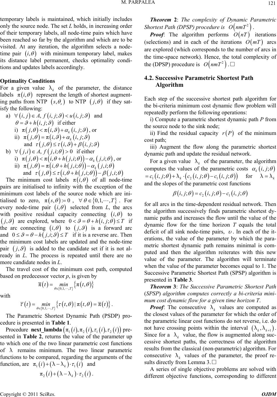

M. PARPALEA 121
whichlly itemporary labels is maintained, initiancludes
only the source node. The set L holds, in increasing order
of their temporary labels, all node-time pairs which have
been reached so far by the algorithm and which are to be
visited. At any iteration, the algorithm selects a node-
time pair

,i

with minimum temporary label, makes
its distance label permanent, checks optimality condi-
tions and us labels accordingly.
Optimality Conditions
pdate
n vaFor a givelue k
λ
of the parameter, the distance
labels

π,i

represent the length of shortest augment-
ing paths from NTP

,

s
s

to NTP


,j

if they sat-
isfy theing:
a)
 
,, ,;ijAfiuij
follow
,;j

  

,hij
and

;

   if either
i)
 


,,
kijπ,πji;

   ,

or
ii)
 


π,ji jπ,,
ki;

  

, ,,ji

;jand i

  
 
,,,;0A fji    if either b)



ji

,

π,,jih i) π,j



; ;
k
ji i

 



π,, ,
k
jihj j
 , or 
ii)

;i

π,;i

    
  
,, ,;,jihji
;
i
and

j

 

 
cost labels

π,i The minimum

of all node-time
e exception of
m
pairs are initialised to infinity with ththe
inimum cost labels of the source node which are ini-
tialised to zero,

π,:0s  ,

0,1, ,T   . For
every node-time pair

,i

selected from L, the arcs
with positive resitydual capaci connecting


,i

to

,j

are explored, w

0,;hij T   here

  if
the arc connecting

,i

to

,j

is a forwarc

;hji T   en
the minimum cost labre up and the node-time
pair
ar
reverse arc. T
d
hand 0,
els a
if it is a
dated

,j

is ad
didate n
ded to the candidate set if it is not al-
ready in L. The process is repeated until there are no
moreodes in L.
The travel cost of the minimum cost path, computed
based on predecessor vector
can
p, is given by




0,1,,
ππ,
T
tmint




with


  
0,1,,,|π,π T
tmint tt  
.
The Patric Shortest Dynamic Path (PSDP) pro-
cedure is ted in Table 1.
 
rame
presen
Procedure next_l ambda



 
1212
π,π,,iiii  pre-
sented in Table 2, returns the value of the parame
ear parametric cost functions
ter up
to which one of the two lin
of
λ
remains minimum. The two linear parametric
functions to be compared, regarding the arguments of the
function, are
  
Theorem 2: The complexity of Dynamic Parametric
Sh
11
πk ii   λλ and
  
i   .
22
πk iλλ
ortest Path (DPSP) procedure is

.
Proof: The algorithm performs iterations
(se
2
OnmT

OnT
lections) and in each of the iterations


T arcs
are explored (which corresponds to the num of rcs in
the time-space network). Hence, the total complexity of
the (DPSP) procedure is
Om
ber a


2
OnmT .□
4.2. Successive Parametric Shortest Path
achsuccessive shortest path algorithm for
the p
Algorithm
step of the E
the bi-criteria minimum cost dynamic flow problem will
repeatedly perform the following operations:
i) Compute a parametric shortest dynamic path P from
the source node to the sink node;
ii) Find the residual capacity

rP of the minimum
cost path;
iii) Augment the flow along arametric shortest
dynamic path and update the residual network.
For a given value k
λ
of the parameter, the algorithm
coof hmputes the values te parametric costs


,;
kij





 


121
,;,; ,;
k
cijc ijcij

  λ for k

λ
λ
and the slopes of the ions parametric cost funct



 
21
,;,; ,;ijcijc ij

 
for all arcs in the time-dependent residual network. Then
the algorithm successively finds parametric shortest dy-
namic paths and increases the flow until the value of the
dynamic flow for the time horizon T equals the total
deficit of all sink node-time pairs,

. In each of the it-
erations, the value of the parameter by which the para-
metric shortest dynamic path remains minimal is com-
puted and then the algorithm reiterates with this new
value of the parameter. The algorithm will terminate
when the value of the parameter becomes equal to 1. The
Successive Parametric Shortest Path (SPSP) algorithm is
presented in Table 3.
Theorem 3: The Successive Parametric Shortest Path
(SPSP) algorithm computes correctly a bi-criteria mini-
mum cost dynamic flow for a given time horizon T.
Proof: The consecutive k
λ
values are computed as
the closest values of the parameter for which the order of
the parametric linear cost functions do not reverse, i.e. do
not have crossing points within the interval


1
,
kk
λλ .
Since for a k
λ
value, the flow is augmented along suc-
cessive shortest paths, the correctness of the algorithm
results from the classical (non-parametric) algorithm. For
consecutive k
λ
values of the parameter, the proof re-
sults directly from Lemma 3.□
A series of single objective problems are solved with
different objective functions, corresponding to different

M. PARPALEA
122
hors t Path (DPSP) procedure. Table 1. Dynamic Parametric S
(1) procedure PSDP
te
),λ,λ,( 1B
kk
p;
(2) beg in
(3) for all T},1,{0,θ do
(4) begin
(5) 0:),(θsπ; 0:),( θsτ;
(6) for all }{-N si do
(7) begin
(8) :),( θiπ; :),( θiτ;
(9) end;
(10) end;
(11) :)(tπ; :)(tτ; }T,1,0,|),({:  θθsL;
(12) while (
 L) do
(13) begin
(14) select ),( i
θi with minimum ),( i θiπ from L; }),({ i θiLL ;
(15) for all (i )

Aj with 0);,( 
i
θjir do
(16) if ));,(( Tθjihθii  then
(17) begin
(18) );,(: iij θjihθθ  ;
(19) 
:λ1k next_lambda )λ,);,(),(,),(,);,α(),( ,),(((1
 kiijiij θjiβθiτθjτθjiθiθjππ;
(20) if ()),();,α(),(( jiiθjθjiθiππ  ) or
))),();,(),(( )),();,α(),(((jiijii θjτθjiβθiτθjθjiθiandππ ) th en
(21) begin
(22) );,α(),(:),( iij θjiθiθjππ; );,(),(:),(iij θjiβθiτθjτ ;
(23) ),(:),( ij θiθjp;
(24) if )),(( Lθjj the n }),({: j
θjLL ;
(25) end;
(26) end;
(27) for all (i)

Aj do
(28) for all j θ such that );,( jji θijhθθ  and );,();,( jjθijuθijr  do
(29) begin
(30) 
:λ1k next_lambda)λ,);,(),( ,),( ,);,α(),( ,),(((1
 kjijjij θijβθiτθjτθijθiθjππ;
(31) if ()),();,α(),(( jji θjθijθiππ  or
))),();,(),(( )),();,α(),(((jjijji θjτθijβθiτθjθijθi andππ )then
(32) begin
(33) );,α(),(:),(jij θijθiθjππ; );,(),(:),(jij θijβθiτθjτ ;
(34) ),(:),( ij θiθjp;
(35) if )),(( Lθjj then }),({:j θjLL ;
(36) end;
(37) end;
(38) end;
(39) }),({)( T},1,{0, θtmintθππ 
; )}(),(),({)(
T},1,{0,
tθt|θtτmintτ
θππ  ;
(40) if ))(( tπ then 0:B
(41) else for all T},1,{0, θ do
(42) 
:λ1knext_lambda )λ,),(,)(( 1
,),(,)(k θtτtτθttππ ;
(43) end;

M. PARPALEA 123
Ta b le 2. P r oc e du r e next_lambda.
(1) procedure next_lambda)λ,)(,)(( 1 ,)(,)( k iτiτii 2121 ππ ;
(2) begi n
(3) 1 λ:λ" k;
(4) if 0))(-)((iτiτ12 then
(5) begin
(6) ))(-)((λ:λ'))/((-)( iτiτii
k1221ππ;
(7) if ()λ '(λk  and )
1
λ '(λ k) th en λ':λ";
(8) end;
(9) return(λ");
(10) end;
Table 3. Successive Parame tric Short est Path (SPSP) algorithm.
(1) SPSP )(G,v;
(2) begin
(3) 0:k; 0:λ
k;
(4) for all T},1,{0, θ do
(5) for all Aji ),( do );,(-);,(:);,( 12 θjicθjicθjiβ;
(6) while 1)(λ
k do
(7) begin
(8) 1:λ
1k ; vv' :;
(9) for all T},1,{0, θ do
(10) for all Aji ),( do
(11) begin
(12) 0:);,( θjifk; ));,();,((λ);,();,(α121 θjicθjicθjicθji kk  ;
(13) end;
(14) while 0)(v' do
(15) begin
(16) 1:B ;
(17) for all T},1,{0,θ do
(18) begin
(19) 0:),(θsp;
(20) for all }{-N si do 1:),( θip;
(21) end;
(22) PSDP),λ,λ,( 1B
kk
p;
(23) if 0)(B then STOP (no path can be found)
(24) e lse
(25) begin
(26) build path P based on p;
(27) });,({:)( ),( i
Pji θjirminPr 
; })(,{:Prv'minδ; v'-δv':;
(28) for all arcs Pji ),( do
(29) begin
(30) if )( ijθθ then δθjirθjir ii -);,(:);,( 
(31) else δθijrθijr jj );,(:);,( ;
(32) compute );,( ik θjif ;
(33) end;
(34) end;
(35) end;
(36) ))}(),({(Y21 kk fyfy:
k;
(37) 1:  kk ;
(38) end;
(39) end;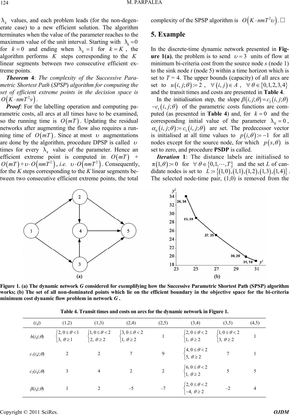

M. PARPALEA
124
k
λ
term
maxi
values, and each problem leads (for the non-degen-
erate case) to a new efficient solution. The algorithm
inates when the value of the parameter reaches to the
mum value of the unit interval. Starting with 0
k

λ
for 0k and ending when for 1
kλkK

, the
K
performs steps
linear segments between two consecutive efficient ex-
treme points.
Theorem 4: The complexity of the Successive Para-
metric Shortest Path (SPSP) algorithm for computing the
t of efficient extreme points in the decision space is
For the labelling operation and computing pa-
rametric costs, all arcs at all times have to be examined,
so the running time is . Updating the residual
networks after augmow also requires a run-
ning time of ost
algorithm Kcorresponding to the
se

2
OKnmTv.
Proof:

OmT
enting the fl
. Since at m

OmT

augmentations
are done by tDPSP is called he algorithm, procedure

times for every k
λ
trem
value of th
com
e eter. Hence
efficient exe point is
param
puted in
an


OmT
onseque
segments be-
+
ntly,

OmT +
for the K

2
OnmT
steps corresp
 ,
on
i.e.  
ding to

2
T
linear
Onm
the K
. C
tween two consecutive efficient extreme points, the total
complexity of the SPSP algorithm is

2
OKnmT

.
rk presented in
3
□
Fig-
5. Example
In the discrete-time dynamic netwo
ure 1(a), the problem is to send

 units of flo
rce node s (nod
e horizon wh
acity) of all ar
w at
e 1)
ich is
cs ar
minimum bi-criteria cost from th
to the sink node t (node 5) with
set to T = 4. The upper bounds (e
set to
e sou
in a tim
cap


,;: 2uij 

,


,ij A


osts are
, 0,1, 2,3  
sented in Table


, 4
4. and the ts and c
lope
ransit timepre


,;j
2
,;ijc i

  In the initialisation step, the s


1,;cij


puted (as pr
of the parametric costs
esented in Table 4) an
corresponding initial value of th
functions are c
for 0 k and
e parameter 0
om-
th
0
d, e

λ,




01
,;c ij,; :ij


m
for the so

is initialised at all ti
nodes except
are set. Th
e values to
urce node,
e predecessor ve

,:1pi   fo
r which
ctor
r all
fo


,ps

is
sed to
set to zero, and procedure PSDP
Iteration 1: The distance labe
is called.
ls are initiali


π1,: 0 

for


0,1, ,T   

and the set L of can-
didate nodes is set to











: 1,0,1L
ode-time pair, (1,0
,.
) is removed from the
1,1,2,1,3,1,4
The selected n
Figure 1. (a) The dynamic network G considered for exemplifying how the Successive Parametric Shor test Path (SP S P) algorithm
works; (b) The set of all non-dominated points which lie on the efficient boundary in the objective space for the bi-criteria
minimum cost dynamic flow problem in network G .
Table 4. Transit times and costs on arcs for the dynamic network in Figure 1.
(i,j) (1,2) (1,3) (2,4) (2,5) (3,4) (3,5) (4,5)
2, 01
3, 1





 1, 02
2, 2





 3, 02
1, 2






1 2, 02
1, 2







1, 02
3, 2





 1
h(i,j;  )
c1(i,j;  ) 2 2 7 9
4, 02
5, 2



 

7 1
c2(i,j;  ) 3 4 2 2
6, 02
1, 2



 

5 5
β(i,j;  ) 1 2 –5 –7
4, 2 
2, 02 




–2 4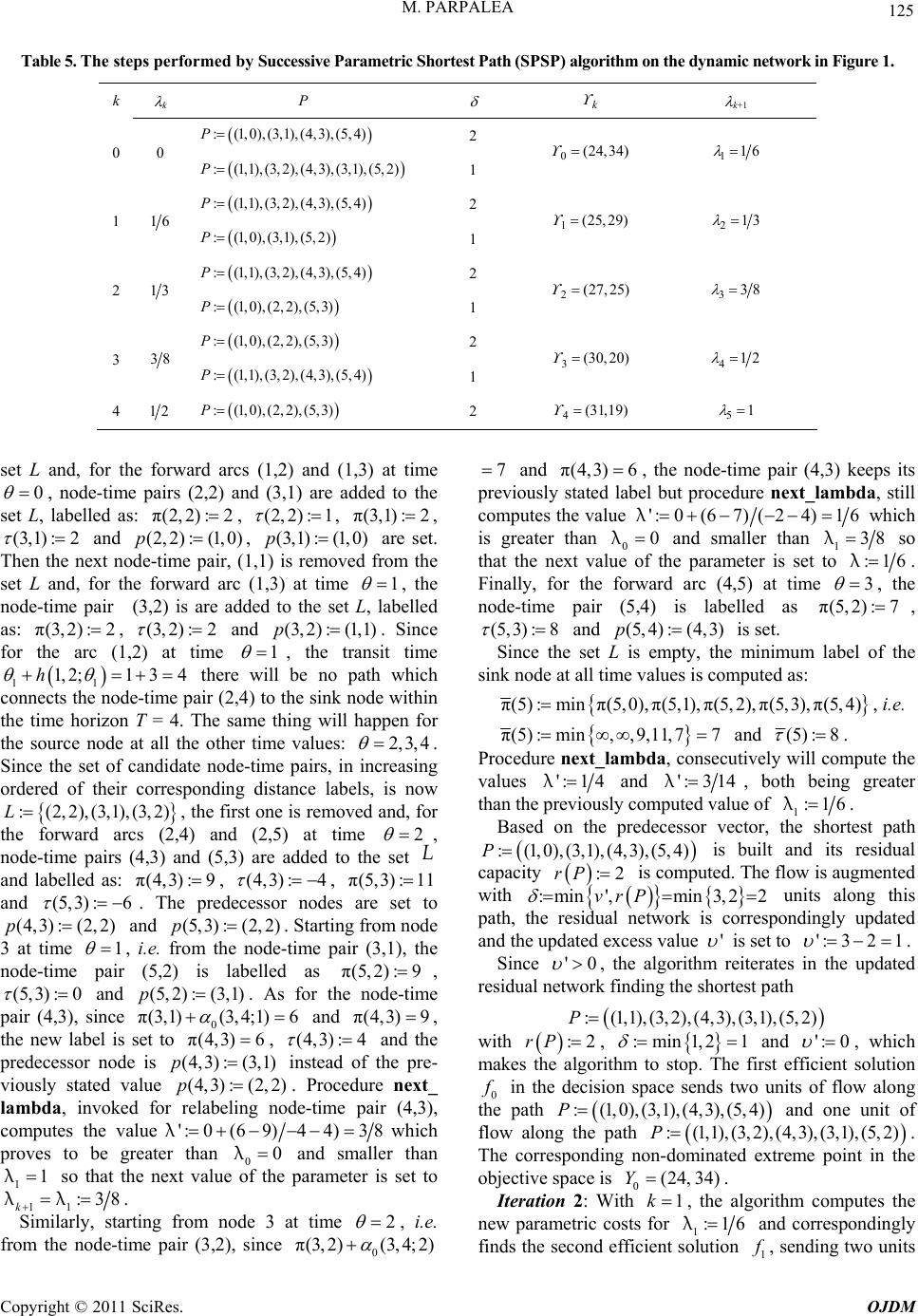

M. PARPALEA 125
test ath (SPSP) algorithm on the dynamic network in Figure 1. Table 5. The steps performed by Successive Parametric Shor
k 
k P
P
 k


k+1


: (1,0),(3,1),(4,3),(5,4)P 2
0 0


: (1,1),(3,2),(4,3),(3,1),(5,2)P0(24,34)
  16
1
 
1


: (1,1),(3,2),(4,3),(5,4)P
1
2
16


: (1,0),(3,1),(5,2)P
1(25, 29)
  213  
1


: (1,1),(3,2),(4,3),(5,4)P 2
2 13


:(1, 0), (2, 2), (5, 3)P
2(27, 25)
  338  
1


), (2, 2), (5, 3)
3
:(1, 0P2
38


: (1,1),(3,2),(4,3),(5,4)P
3(30, 20)
  412  
1
4 12


:(1, 0), (2, 2), (5,3)P 4(31,19)   51  
2
d,ward ad (1,3) at time
0
set L an for the forrcs (1,2) an

, node-time pairs (2,2) and (3,1) are added to the
set L, labelled as: π(2,2) :2, (2,2) :1

, π(3,1):2

,
(3,1):2

 and (2,2):(1,0)p, (3p.,1):(
,1) is rem
(1,3) at time
1,0) are set
oved from the
1
xt no
for th
Then t
set L
he ne
and,
de-time pair, (1
e forward arc


, the
t L, labelled e pair node-tim
as: π(3
(3,2) is are adde
(3, 2):2
d to the se
, 2) :2,


) at time
and
,2
(3,2):p
1
(1,1) . Since
for the arc (1


will be
) to the si
me
time values:
, the transit time
no path which
nk node within
thing will happen for
2,3,4

11

e node
horizon
1, 2; 
h
e
rc
1
T
e node at all th
3 4 there
-time pair (2,4
= 4. The sa
e other
h
connects t
the tim
the sou


.
in increasing
bels, is now
oved and, for
me 2
Since the
ordere
: (L
the fo
set of candidate nod
rresponding

3,2) , the first
2,4) and (
e-time pairs,
distance la
one is rem
2,5) at ti
d of
2,2)
rwar
thei
,(3,1)
d
r co
,(
arcs (


,
o the set L node-time pairs (4,3) and (5,3) are added t
and labelled as: π(4,3):9, (4,3) :4

 , π(5,3):11

and (5,3):6

 . The predecessor nodes are set to
(4,3) :(2,2)p and (5,3):(2,2)p

. Starting from node
3 at time 1


e pair (
, i.e. from th
5,2)
e node-time pair (3,1), the
is labelled as π(5, 2) :9 node-tim

,
(5,3) :0


,3),
a
since
nd (5,2):)p
0
(3,1) (3,
(3,1. As f
;1)6
or the node-time
pair (4π4

 and π(4,3) 9

,
the new label is set to π(4,3) 6

, (4,3) :4

 and the
predecessor node ( is (4,3) :p3,1)

instea
(2,2)
d of the pre-
viously stated value (4,3) :p

. Proc
ling node-tim
edure next_
e pair (4,3),lambda
com
, in
putes the
voked for relabe
value': 0(6λ
ter than λ
ext value
9) 44)3 
0 and smalle
he parameter is
8 wh
set
ich
r than
to
proves to
11λ
be grea0
at the n so thof t
1k
λ
Sim
1
:λ
ilarly,
38.
startin

g from node 3 at time 2


, i.e.
from the node-time pair (3,2), since 0
π(3, 2)(3, 4;2)


7

and π(4,3) 6

, the node-time pair (4,3) keeps its
tated ure next_lambda, still
computes the value
previouslybut proced slabel
':0(67)(24)16

 λ
is greater than 00
which

λ and smaller than 138

λ so
that the nehe parameter is set to xt value of t:16

λ.
Finally, fod arc (4,5) at time r the forwar3


, the
-tim is labelled as nodee pair (5,4)π7(5,2):

,
(5,3) :8


and (5,p4) :(4,3)

is set.
inimum
puted as:
Since the set L is em
sink node at all time
pty, the m
values is com
label of the


(5, 4),π(5):min π(5,0), π(5,1), π(5,2), π(5,3), π i.e.


, 77 and π(5):min,,9,11

 (5) :8


pute the
.
comProcedure , consecutively will
values
next_lambda
':14

λ and ': 314

λ, both b
than thf
eeatering gr
e previously computed value o1 λ
h
:16.
e shortest pathBased vector, t on the predecessor


: (1,0),(3,1),4)P is built and its residual ,(4,3),(5
capacity


:2rP

is computed. The flow is augmented
with





:min',min3,22vrP 


units along this
path, the resiork is
and the updated evalue
dual netw
xcess
corresp
'
ondi ngly updated

is set to ': 321


.
Since '0

, the algorithm reiterates in th
residuetwor the shath
e updated
al nk findingortest p


) : ,2),(4,3),(3,1),(5,2P(1,1),(3
with


:2rP

,


in1,21 and :m 

': 0

, which
ution ma kes the algorithm to stop. The first efficient sol
0
f
in the
the path
decision space sends two units of flow along


) :P
along th
(1,0),(3,1
e path
),(4,3),(5,4 and one unit of
flow


),(3,1),(5,2)
int in th
: (1,1),(3,
dominad
(24,34)
2),(
ex
4.
treme
,3P
ing non-
is 0 Y
The correspond
space
tee po
objective

.
1 Iteration 2: With k

, thle agorithm computes the
new parametric costs for 1:16λ and co rrespondingly
finds the second efficient solution 1
f
, sending two units

M. PARPALEA
126
of flow along t pat and
one unit of flow alo
with the extree point
heh

:(1,1),(3,2) 4,3),(5,4)P
ng the path : (1,0),(3,1),(5,P
in the objective space
,(

2) ,
1
Y m

(25,29) , and 2:13.
ed by the algorithm are describe
space with the non-doi
ted in Figure 1(b).
gnanti and J. Orlin, “Network Flows.
s and Applications,” Prene Hall,
, New Jersey, 1993.
of Dynamic Network
, Vol. 1, No.1, 1

steps perform
nd the objective
e points is prese
R. Ahuja, T. Ma
y, Algorithm
Englewood Cliffs
J. A. Aronson, “A Survey
Annals of Operations Research
λ
The
Table 5 a
extrem
6. References
[1]
Theor
[2]
d in
nated
Inc.
Flows,”
989, pp.
,
m
n
tic
1-66. doi:10.1007/BF02216922
[3] W.
T
agem
Chin
Powell, P. Jaillet and A. Odoni, “Stochastic
ooks in Operations Research and
e, Chapter 3, North Holland, A
Kaw
on
&
a, 2009, pp. 453-
I. Chabini and M. Abou-Zeid, “Tost Flow
Problem in Capacitated Dynamic Networks,” Annual
Meeting of the Transportation Research Board, Wash-
ington, D.C., 20. 1-30.
E. Nasrabadi and S. M. Hashemi, “Minimum Cost Time-
Varying Network Flow Problems,” Optimization Methods
and Software, V, No. 3, 2010, pp. 429-447.
and Dy-
Man
namic Networks and Routing,” In: Ball, M. O., Magnanti,
. L., Monma, C. L. and Nemhauser G. L., Ed., Network
Routing, Handb-
ent Sciencmsterdam,
The Netherlands, Vol. 8, 1995, pp. 141-295.
[4] N. Kamiyama, A. Takizawa, N. Katoh and Y. abata,
“Evaluation of Capacities of Refuges in Urban Areas by
Using Dynamic Network Flows,” Proceedings of the
Eighth International Symposium Operations Research
and Its Applications, ORSCAPORC, Zhangjiajie,
460.
[5] he Minimum C
03, pp
[6]
ol. 25
doi:10.1080/10556780903239121
H. Lee and S. Pulat, “Bicriteria Network Flow Problems:
Continuous CasEuropean Journal of Operational Re-
search, Vol. 51, No. 1, 1991, pp. 119-126.
[7]
e,”
doi:10.1016/0377-2217(91)90151-K
S. Gass and T. Sy, “The Computational Algorithm for
the Parametric Objective Function,” Naval Research Lo-
gistics Quarterly, No. 1-2, 1955, pp. 39-45.
[8] aat
, Vol. 1
doi:10.1002/nav.3800020106
[9] A. M. Geoffrion, “Solving Bicriterion Mathematical Pro-
grams,” Operations Research, Vol. 15, No. 1, 1967, pp.
39-54. doi:10.1287/opre.15.1.39
d K.ransporta
1979, p
[10] Y. P. Aneja an P. Nair, “Bicriteria Ttion
Problem,” Management Science, Vol. 25, No. 1,p.
73-78. doi:10.1287/mnsc.25.1.73
[11] A. Skriver, “A Classification of Bicriterionh
ific Journal
Shortest Pat
(BSP) Algorithms,” Asia-Pac of Operational
ying Network
Research, No. 17, 2000, pp. 199-212.
[12] X. Cai, D. Sha and C. Wong, “Time-Var
Optimization,” Springer, New York, 2007.