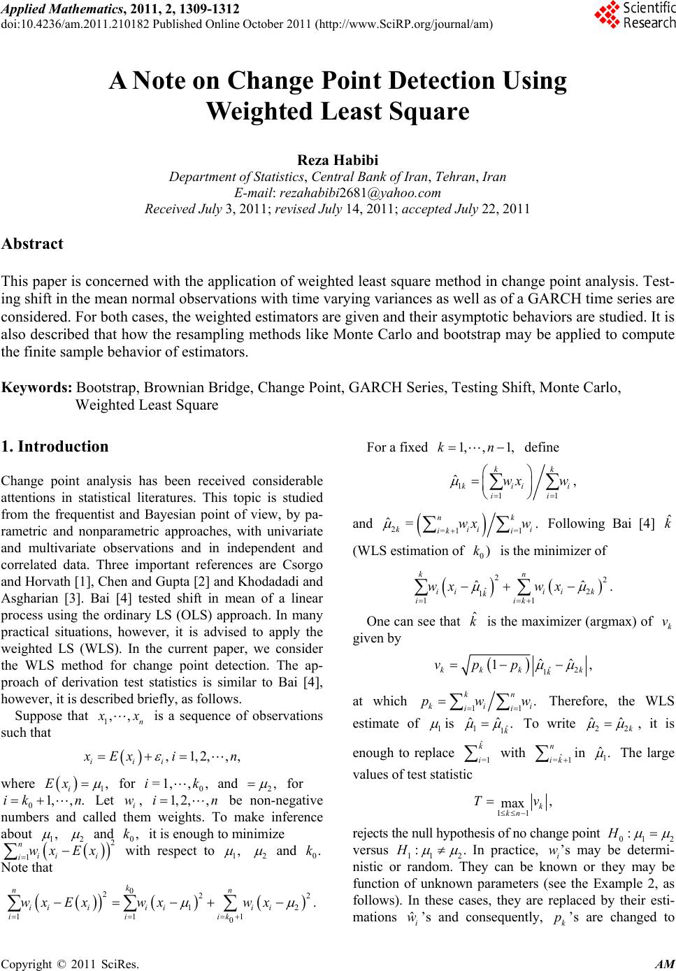
Applied Mathematics, 2011, 2, 1309-1312
doi:10.4236/am.2011.210182 Published Online October 2011 (http://www.SciRP.org/journal/am)
A Note on Change Point Detection Using
Weighted Least Square
Reza Habibi
Department of St at istics, Central Bank of Iran, Tehran, Iran
Received July 3, 2011; revised July 14, 2011; accepted July 22, 2011
Abstract
This paper is concerned with the application of weighted least square method in change point analysis. Test-
ing shift in the mean normal observations with time varying variances as well as of a GARCH time series are
considered. For both cases, the weighted estimators are given and their asymptotic behaviors are studied. It is
also described that how the resampling methods like Monte Carlo and bootstrap may be applied to compute
the finite sample behavior of estimators.
Keywords: Bootstrap, Brownian Bridge, Change Point, GARCH Series, Testing Shift, Monte Carlo,
Weighted Least Square
1. Introduction
Change point analysis has been received considerable
attentions in statistical literatures. This topic is studied
from the frequentist and Bayesian point of view, by pa-
rametric and nonparametric approaches, with univariate
and multivariate observations and in independent and
correlated data. Three important references are Csorgo
and Horvath [1], Chen and Gupta [2 ] and Khodadad i and
Asgharian [3]. Bai [4] tested shift in mean of a linear
process using the ordinary LS (OLS) approach. In many
practical situations, however, it is advised to apply the
weighted LS (WLS). In the current paper, we consider
the WLS method for change point detection. The ap-
proach of derivation test statistics is similar to Bai [4],
however, it is described briefly, as follows.
Suppose that 1,,
n
x
x is a sequence of observations
such that

,1,2,,
iii ,
x
Ex in  
where

1, i
Ex

 for and 20 =1,, ,ik,


n for
0 Let i, be non-negative
numbers and called them weights. To make inference
about
1,, .n
1,
ik w1, 2,,i

2

and 0 it is enough to minimize
1i with respect to
,k



2
ii i
wx Ex
n
1,

2

and
Note that 0.k
   
0
22
1
111
0
.
k
n
ii iiiii
iiik
wx Exwxwx 

 

For a fixed 1, ,1,kn

 define
111
ˆ,
kk
kii
ii
wx w 




i


and

 2=1 =1
ˆ=
n
kii
ik i
wx w 


.
k
i
Following Bai [4]
(WLS estimation of is the minimizer of
ˆ
k
0)k


22
ˆ2
1
11
ˆˆ .
kn
iiii k
k
iik
wx wx 

 

One can see that is the maxi mizer ( arg max) o f
given by
ˆ
kk v

ˆ2
1
ˆˆ 1,
kkk k
k
vpp   
at which 11 .
kn
ki
ii
pw


i
w
Therefore, the WLS
estimate of 1

is ˆ
11
ˆˆ
.
k



To write 22
ˆˆ
k

 , it is
enough to replace ˆ
=1
k
i

with in
ˆ
=1
n
ik
1
ˆ.

The large
values of test statistic
11
,
max k
kn
Tv


2
2
n

rejects the null hypothesis of no change point 01 2
:H



versus 11 2
:
.
H



In practice, i’s may be determi-
nistic or random. They can be known or they may be
function of unknown parameters (see the Example 2, as
follows). In these cases, they are replaced by their esti-
mations ’s and consequently, ’s are changed to
w
k
p
ˆi
w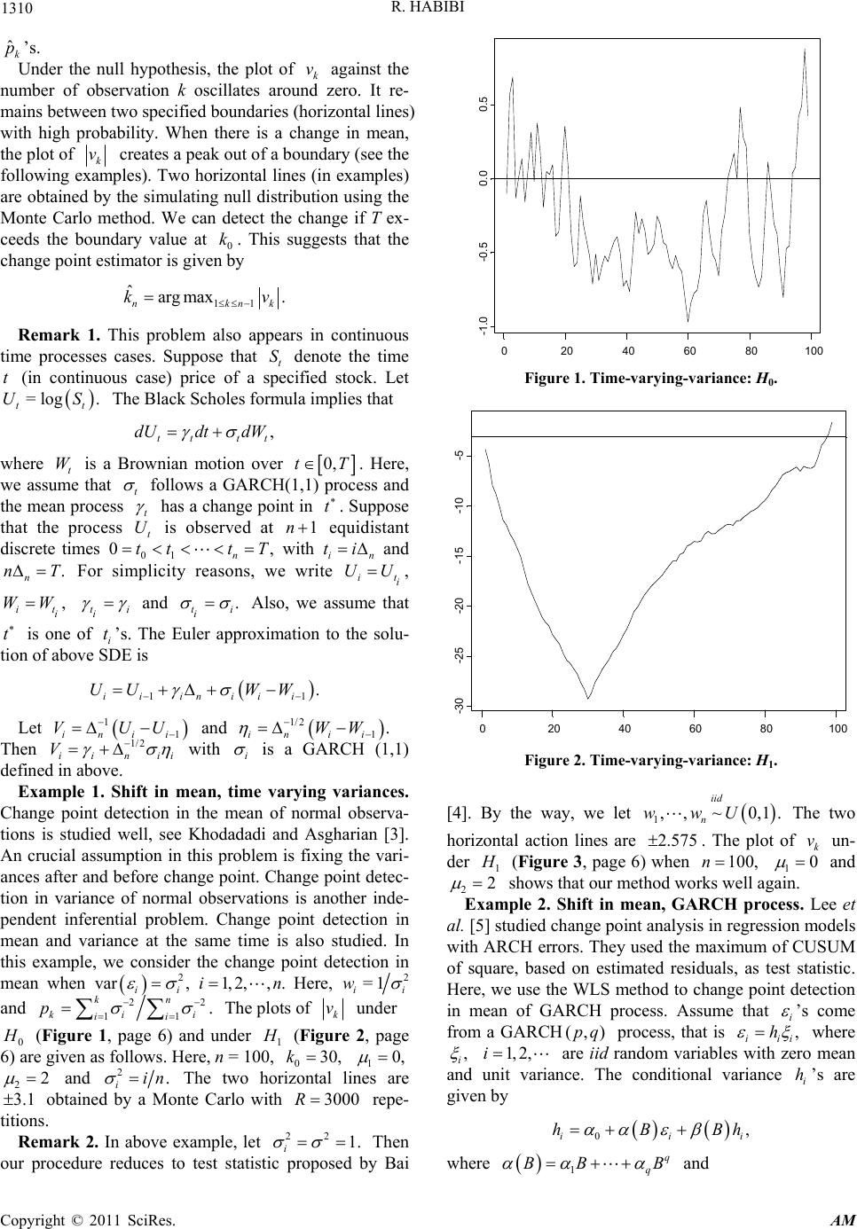

1310 R. HABIBI
ˆk p’s.
Under the null hypothesis, the plot of k against the
number of observation k oscillates around zero. It re-
mains between two specified boundaries (horizontal lines)
with high probability. When there is a change in mean,
the plot of
v
k
v creates a peak out of a boundary (see the
following examples). Two horizontal lines (in examples)
are obtained by the simulating null distribution using the
Monte Carlo method. We can detect the change if T ex-
ceeds the boundary value at 0. This suggests that the
change point estimator is given by
k
11
ˆargmax .
nkn
kv

k
t
Remark 1. This problem also appears in continuous
time processes cases. Suppose that t denote the time
(in continuous case) price of a specified stock. Let
The Black Scholes formula implies that
S
t

= log.
t
US
,
tt tt
dUdt dW

 
where t is a Brownian motion over W


0,tT. Here,
we assume that t

follows a GARCH(1,1) process and
the mean process t

has a change point in . Suppose
that the process is observed at equidistant
discrete times 0, with n
t
t
1n
t

U
01 ni
tt tT i


U
and
.T
n
n For simplicity reasons, we write it
i
U

,
,
it
i
WWt
ii

  and .
t
ii

  Also, we assume that
t is one of i t’s. The Euler approximation to the solu-
tion of above SDE is

11
.
ii iniii
UU WW 


Let and
Then

11inii
VUU


 
1/2
iinii
V

1/2 1.
in ii
WW 


 



 with i

is a GARCH (1,1)
defined in above.
Example 1. Shift in mean, time varying variances.
Change point detection in the mean of normal observa-
tions is studied well, see Khodadadi and Asgharian [3].
An crucial assumption in this problem is fixing the vari-
ances after and before change point. Change point detec-
tion in variance of normal observations is another inde-
pendent inferential problem. Change point detection in
mean and variance at the same time is also studied. In
this example, we consider the change point detection in
mean when

2
var ,
ii

  Here, 1, 2,,.in2
=1
i
wi

and 2
k



2
.
n


11
kii
ii
p  The plots of k v under
0
H
(Figure 1, page 6) and under 1
H
(Figure 2, page
6) are given as follows. Here, n = 100, 0 1
30,k0,


22

 and 2.
iin
  The two horizontal lines are
obtained by a Monte Carlo with repe-
titions.
3.13000R
Remark 2. In above example, let Then
our procedure reduces to test statistic proposed by Bai
22
1.
i
 
0 20406080100
-1.0 -0.50.00.5
Figure 1. Time-varying-variance: H0.
0 20406080100
-30 -25 -20 -15 -10-5
Figure 2. Time-varying-variance: H1.
[4]. By the way, we let The two

1,, ~0,1.
iid
n
wwU
horizontal action lines are . The plot of un-
der 2.575k
v
1
H
(Figure 3, page 6) when 1 100,n0


and
22


shows that our method works well again.
Example 2. Shift in mean, GARCH process. Lee et
al. [5] studied change point analysis in regression models
wit h ARC H erro rs. They u sed t he max imum o f CU SUM
of square, based on estimated residuals, as test statistic.
Here, we use the WLS method to change point detection
in mean of GARCH process. Assume that i

’s come
from a GARCH process, that is iii
(,)pq ,h

  where
,
i

1, 2,i

 are iid random variables with zero mean
and unit variance. The conditional variance ’s are
given by i
h


0, ii
hBB    i h
where


1q q
BB B    and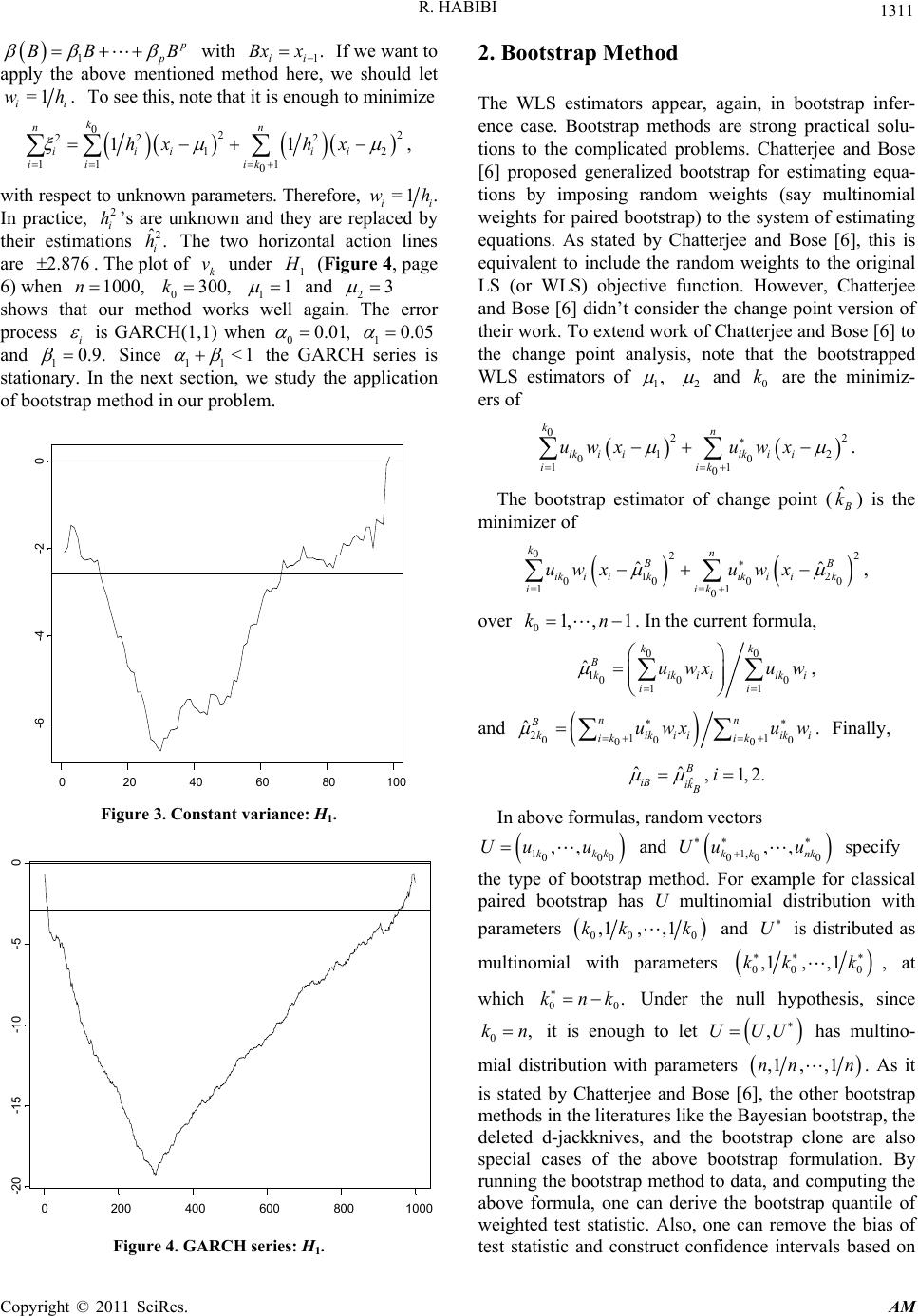

R. HABIBI
1311

1
p
p
BB B    with 1 If we want to
apply the above mentioned method here, we should let
.
ii
Bxx 
=1 .
ii
wh To see this, note that it is enough to minimize




02
22 2
1
11 1
0
11
k
nn
iii ii
ii ik
hx hx 
 

 2
2
, 
with respect to unknown parameters. Therefore, =1
ii
wh.
In practice, ’s are unknown and they are replaced by
their estimations The two horizontal action lines
are . The plot of under 1
2
i
h2
ˆ.
i
h
2.876k v
H
(Figure 4, page
6) when 0 1
1000, kn 300,1

 and 23


shows that our method works well again. The error
process i

is GARCH(1,1) when 00.01

, 10.05


and 10.9.

 Since 11 <1

  the GARCH series is
stationary. In the next section, we study the application
of bootstrap method in our problem.
020406080100
-6 -4 -20
Figure 3. Constant variance: H1.
0200 400 600 8001000
-20 -15 -10-50
Figure 4. GARCH series: H1.
2. Bootstrap Method
The WLS estimators appear, again, in bootstrap infer-
ence case. Bootstrap methods are strong practical solu-
tions to the complicated problems. Chatterjee and Bose
[6] proposed generalized bootstrap for estimating equa-
tions by imposing random weights (say multinomial
weights for paired bootstrap) to the system of estimating
equations. As stated by Chatterjee and Bose [6], this is
equivalent to include the random weights to the original
LS (or WLS) objective function. However, Chatterjee
and Bose [6] didn’t consider the change point version of
their work. To extend work of Chatterjee and Bose [6] to
the change point analysis, note that the bootstrapped
WLS estimators of ,
1

2

and 0 are the minimiz-
ers ofk
 
022
12
00
11
0
.
kn
ik iiik ii
iik
uwx uwx 




The bootstrap estimator of change point (ˆ
B
k) is the
minimizer of
 
022
12
00 0
=1=1
0
ˆˆ ,
kn
BB
ik iikik iik
iik
uwx uwx 


 
 
0
over 01, ,1kn

. In the current formula,
00
100 0
11
ˆ,
kk
B
kikii iki
ii
uwxuw 






and

 21
00
00
ˆ.
nn
B
kikii iki
ik ik
uwxuw 

 

1
0
Finally,
ˆ
ˆˆ
,1,2
B
iB ik Bi
  .
In above formulas, random vectors

 100
,,
kkk
Uu u0 and specify
the type of bootstrap method. For example for classical
paired bootstrap has U multinomial distribution with
parameters
 1,
00 0
,,
kk nk
Uu u
 



00 0
,1, ,1kk k and U is distributed as
multinomial with parameters


00 0
,1,,1kk k
 
, at
which 00 .knk


 Under the null hypothesis, since
0,kn

it is enough to let has multino-
mial distribution with parameters

,UUU




,1 ,,1nn n. As it
is stated by Chatterjee and Bose [6], the other bootstrap
methods in the literatures like the Bayesian bootstrap, the
deleted d-jackknives, and the bootstrap clone are also
special cases of the above bootstrap formulation. By
running the bootstrap method to data, and computing the
above formula, one can derive the bootstrap quantile of
weighted test statistic. Also, one can remove the bias of
test statistic and construct confidence intervals based on

R. HABIBI
1312
bootstrap, we have done these calculations and it has
been seen that the results are very good. Interested reader
can refer to Habibi [7].
3. References
[1] M. Csorgo and L. Horvath, “Limit Theorems in Phange-
Point Analysis,” Wiley & Sons, New York, 1997.
[2] J. Chen and A. K. Gupta, “Parametric Statistical Change
Point Analysis,” Birkhäuser, Basel, 2000.
[3] A. Khodadadi and M. Asgharian, “Change Point Problem
and Regression: An Annotated Bibliography,” Technical
Report, McGill University, Montreal, 2004.
[4] J. Bai, “Least Squares Estimation of a Shift in Linear
Processes,” Journal of Time Series Analysis, Vol. 15, No.
5, 1994, pp. 453-472.
doi:10.1111/j.1467-9892.1994.tb00204.x
[5] S. Lee, Y. Tokutsu and K. Maekawa, “The CUSUM Test
for Parameter Change in Regression Models with ARCH
Errors,” Journal of Japan Statistical Society, Vol. 3, 2004,
pp. 173-186.
[6] S. Chatterjee and A. Bose, “Generalized Bootstrap for
Estimating Equations,” Annals of Statistics, Vol. 33, No.
1, 2005, pp. 414-436. doi:10.1214/009053604000000904
[7] R. Habibi, “Change Point Detection Using Weighted
Least Square,” Technical Report, Central Bank of Iran,
2010.