Applied Mathematics, 2011, 2, 1303-1308
doi:10.4236/am.2011.210181 Published Online October 2011 (http://www.SciRP.org/journal/am)
Independence of the Residual Quadratic Sums in the
Dispersion Equation with Noncentral χ2-Distribution
Nikolay I. Sidnyaev, Kristina S. Andreytseva
Bauman Moscow State Technical University, Moscow, Russia
Received May 6, 2011; revised July 1, 2011; accepted July 8, 2011
Abstract
A model adequacy test should be carried out on the basis of accurate aprioristic ideas about a class of ade-
quate models, as in solving of practical problems this class is final. In article, the quadratic sums entering
into the equation of the dispersive analysis are considered and their independence is proved. Necessary and
sufficient conditions of existence of adequate models are resulted. It is shown that the class of adequate
models is infinite.
Keywords: Noncentral χ2-Distribution, Dispersion Analysis, Adequate Models, Quadratic Sums
1. Introduction
The dispersive analysis is defined as the statistical method
intended for estimation of influence of various factors on
a result of experiment, so application area of this method
becomes much wider. Unbiased estimate for unknown
parameters is the sum of squares. The main idea of the
dispersive analysis consists in splitting of this sum of
squares of deviations into some components, each of
which corresponds to the prospective reason of averages
changing.
Let’s consider decomposition of the residual sum of
squares
01
QQQ
2
and we will prove independence of the summands Q1 and
Q2. Two theorems and four auxiliary lemmas will be
necessary for the proof.
2. Preliminaries
Lemma 2.1. The rank of composition of two matrixes A
and B is less or equal to minimal rank of matrixes A and
B i.e.


 
min, .rABrA rB
Proof. By a rule of matrixes multiplication, columns
of matrix AB are a linear combination of columns of a
matrix A, then the number of linearly independent col-
umns in AB can’t surpass the number of linearly inde-
pendent columns in A; consequently


rAB rA

.
Doing similar reasoning for the lines (the lines of AB
are a linear combination of the lines B), we will receive
that




rAB rB. The lemma is proved.
Consequence of the inertia law of square-law forms
(about quantity of invariants): if QxAx


n
is the
square-law form with n variables 1,
x
x and its rank
is equal to r,


rA r

, then r linear combinations of
variables 1,n
x
x exist, for example, such
1,,zr
z
that 2
1
ii
i
Q
r
z


 and every 1
i

 or . 1
s
We will use the Kohran theorem as a simple conse-
quence of the following theorem.
Theorem 2.1. Let , where
2
1
1
N
i
i
yQ Q



j
Q,
1,js

, are the square-law form with rank
j
n from vari-
ables 1,,
N
yy. Then the condition 12 s nn n
N

Ay
is a necessary and sufficient condition for existence of
the orthogonal transformation translating a vec-
tor
z

1,,yy

N
y

 into a vector

,,
N
z
1
zz

 in
such way, that
1 112
11
...
22
12
11... 1
,,,
s
s
nn nnn
iis
iin inn
QzQ zQz

 
 
 
 

1
2
,
i
Prove. Necessity.
If such orthogonal transformation exists, then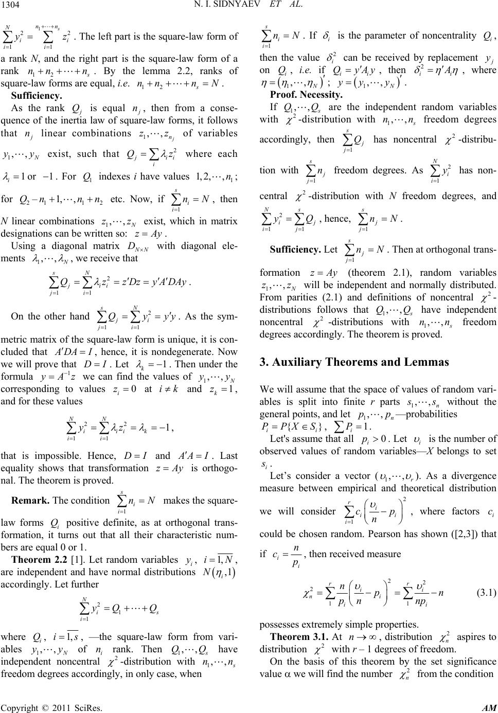

1304
2
i
z
N. I. SIDNYAEV ET AL.
1
2
11
s
nn
N
i
ii
y





. The left part is the square-law form of
a rank N, and the right part is the square-law form of a
rank 12
s
nn n. By the lemma 2.2, ranks of
square-law forms are equal, i.e. .
12 s
nnn N
Sufficiency.
As the rank
j
Q is equal
j
n, then from a conse-
quence of the inertia law of square-law forms, it follows
that
j
n linear combinations 1,,
j
n
zz of variables
1,,
N
yy exist, such that 2
j
ii
i
Qz

 where each
1
i

or . For indexes i have values ;
for – etc. Now, if , then
1
n
1
Q
n
1
1, 2,, n
nN
2
Q11 1, ,2 n
1
s
i
i
N linear combinations 1,,
N
zz exist, which in matrix
designations can be written so: .
zAy
Using a diagonal matrix
N
N
D with diagonal ele-
ments 1,,
N

 , we receive that
2
11
sN
jii
ji
QzzDzyAD 

 
 Ay
y
.
On the other hand . As the sym-
2
11
sN
ji
ji
Qyy




metric matrix of the square-law form is unique, it is con-
cluded that
A
DA I

D
, hence, it is nondegenerate. Now
we will prove that . Let I1
k

 . Then under the
formula 1
y
Az

 we can find the values of 1,,
N
yy
corresponding to values 0
i
z

at and ik1
k
z

,
and for these values
22
11
1
NN
iiik
ii
yz 


 ,
that is impossible. Hence, and
DI
A
AI


. Last
equality shows that transformation is orthogo-
nal. The theorem is proved.
zAy
Remark. The condition makes the square-
1
s
i
i
nN



law forms i positive definite, as at orthogonal trans-
formation, it turns out that all their characteristic num-
bers are equal 0 or 1.
Q
Theorem 2.2 [1]. Let random variables i, y1,iN,
are independent and have normal distributions


,1
i
N 
accordingly. Let further
2
1
1
N
is
i
y
QQ



where ,
i
Q1,i
1
s
i
i
nN


. If i

is the parameter of noncentrality ,
i
Q
then the value i
2

can be received by replacement
j
y
on , i.e. if
i
Qii QyAy


, then 2
ii
A



, where

,,
N

1


; .

N
y

1,,yy

Proof. Necessity.
If 1,,
s
QQ
2
are the independent random variables
with

-distribution with 1,,
s
nn freedom degrees
accordingly, then
1
s
j
j
Q


has noncentral 2

-distribu-
tion with
1
s
j
j
n


freedom degrees. As has non-
central
2
i
y
1
N
i

2

-distribution with N freedom degrees, and
2
y
11
j
Q
Ns
i
ij 

, hence, .
1
s
j
j
nN
Sufficiency. Let
1
s
j
j
nN


. Then at orthogonal trans-
formation zAy

(theorem 2.1), random variables
1,,
N
zz will be independent and normally distributed.
From parities (2.1) and definitions of noncentral 2

-
distributions follows that 1,,
s
QQ have independent
noncentral 2

-distributions with 1,,
s
nn freedom
degrees accordingly. The theorem is proved.
3. Auxiliary Theorems and Lemmas
We will assume that the space of values of random vari-
ables is split into finite r parts 1,,
n
s
s without the
general points, and let —probabilities
1,, n
pp
{}
ii
PPXS

, 1
i
P


.
Let's assume that all i. Let i 0p

is the number of
observed values of random variables—X belongs to set
i
s
.
Let’s consider a vector (1,,
r

 ). As a divergence
measure between empirical and theoretical distribution
we will consider
2
1
r
i
ii
i
cp
n








, where factors
could be chosen random. Pearson has shown ([2,3]) that
if
i
c
i
i
n
cp , then received measure
22
2
11
rr
i
ni
ii
np
pn np


 i
n

 



(3.1)
possesses extremely simple properties.
s, —the square-law form from vari-
ables 1,,
N
yy of i rank. Then 1 n,,
s
QQ have
independent noncentral 2

-distribution with 1,,
s
nn
freedom degrees accordingly, in only case, when
Theorem 3.1. At , distribution n 2
n

aspires to
distribution 2

with r – 1 degrees of freedom.
On the basis of this theorem by the set significance
value  we will find the number 2
n

from the condition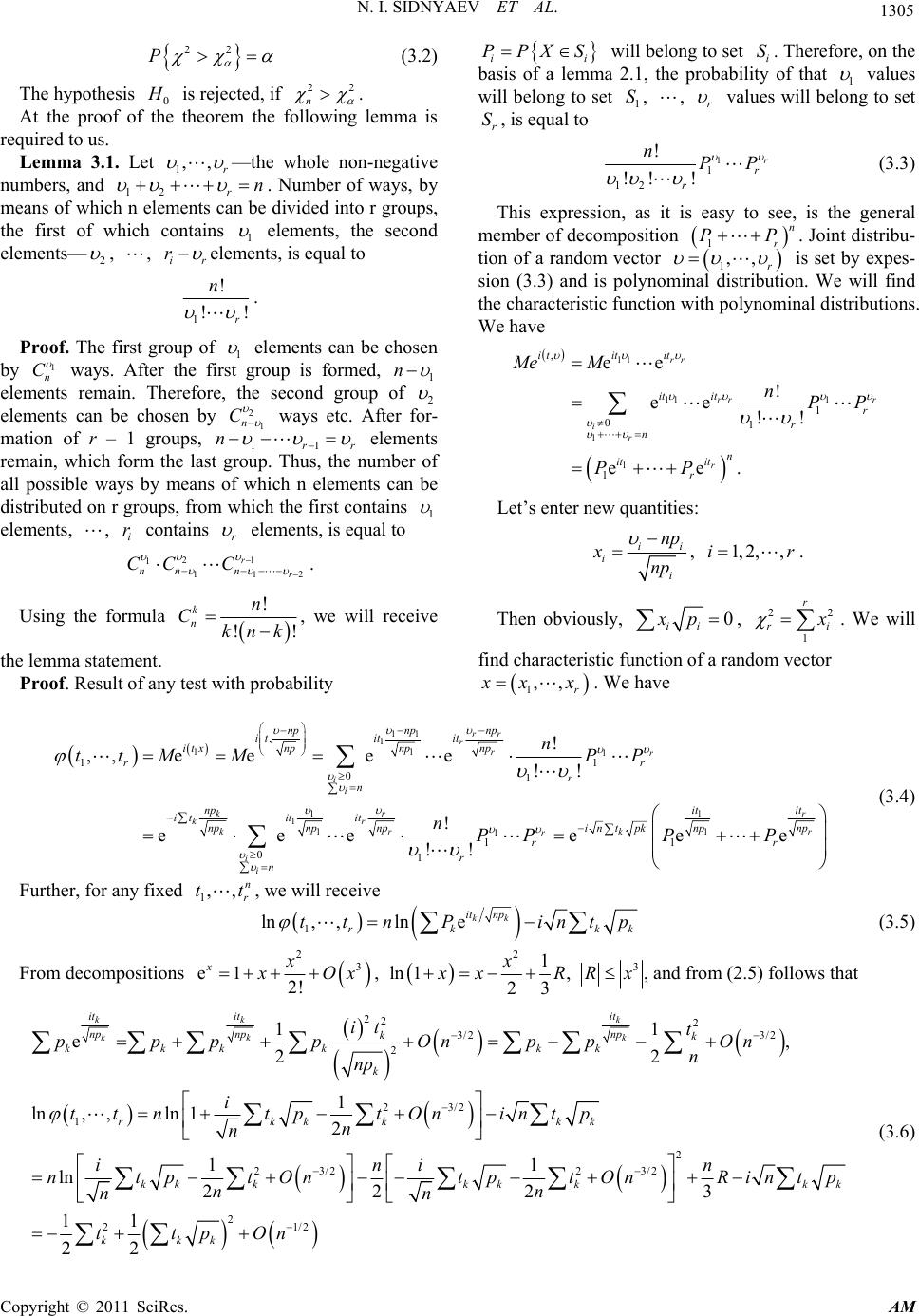

N. I. SIDNYAEV ET AL.
1305

22
P


  (3.2)


i
PPXS
i
will belong to set i. Therefore, on the
basis of a lemma 2.1, the probability of that 1
S

values
will belong to set , ,
1
Sr

values will belong to set
, is equal to
r
S
The hypothesis 0
H
is rejected, if 22
n


 .
At the proof of the theorem the following lemma is
required to us.
1
1
12
!
!! !
r
r
r
nPP


 

 (3.3)
Lemma 3.1. Let 1,,
r

 —the whole non-negative
numbers, and 12rn

   . Number of ways, by
means of which n elements can be divided into r groups,
the first of which contains 1

elements, the second
elements— 2

, , ir r

elements, is equal to
This expression, as it is easy to see, is the general
member of decomposition . Joint distribu-
tion of a random vector

1
n
r
PP

1,, r



  is set by expes-
sion (3.3) and is polynominal distribution. We will find
the characteristic function with polynominal distributions.
We have
1
!
!!
r
n

 .
Proof. The first group of 1

elements can be chosen
by 1
n
C

ways. After the first group is formed, 1 n


elements remain. Therefore, the second group of 2

elements can be chosen by 2
1
n
C


 ways etc. After for-
mation of r – 1 groups, 11rr n




 elements
remain, which form the last group. Thus, the number of
all possible ways by means of which n elements can be
distributed on r groups, from which the first contains 1

elements, , contains i rr

elements, is equal to


11
11 1
1
1
,
1
01
1
ee
!
ee !!
ee.
rr
rr r
i
r
r
it it it
it it
r
r
n
n
it it
r
Me M
nPP
PP







 










Let’s enter new quantities:
ii
i
i
np
xnp
 
, . 1,2,,ir
21 1
11
r
r
nnn
CC C
 




 
2
.
Using the formula

!
!!
k
n
n
Cknk , we will receive Then obviously, 0
ii
xp

, 2
1
r
r
2
i
x
 . We will
find characteristic function of a random vector the lemma statement.


1,, r
x
xx. We have Proof. Result of any test with probability


11
1
11 1
1 1
1
1 1 1
,
1 1
01
11
01
!
,, eeee!!
!
eee ee
!!
rr
r
rr
i
i
kr r
kr
kr r k r
i
i
npnp np
it it it
np itxnp np
r r
r
n
np it it
it it it
np np npnpnp in tpk
rr
r
n
n
ttMMPP
nPPPP



















 


 






 
e
(3.4)
Further, for any fixed , we will receive
1,,
n
r
tt


 1
ln,,lne kk
it np
rk k
ttn Pintp  

k (3.5)
From decompositions

2
3
e1 2!
xx
x
Ox,

21
ln 123
x
x
xR, 3 Rx, and from (2.5) follows that


 


 
222
3/2 3/2
2
23/2
1
2
23/2 23/2
11
e ,
22
1
ln,,ln 12
11
ln 2223
kk k
kk k
it itit
np npnp kk
kkk kkk
k
rkkk kk
kkkkk k
it t
ppppOnp pOn
n
np
i
ttntptOn intp
n
n
ini n
ntptOntptOn Rin
nn
nn




  

 


 

 
 
  
 
 



2
21/2
11
22
kk
kkk
tp
ttpOn

 


(3.6)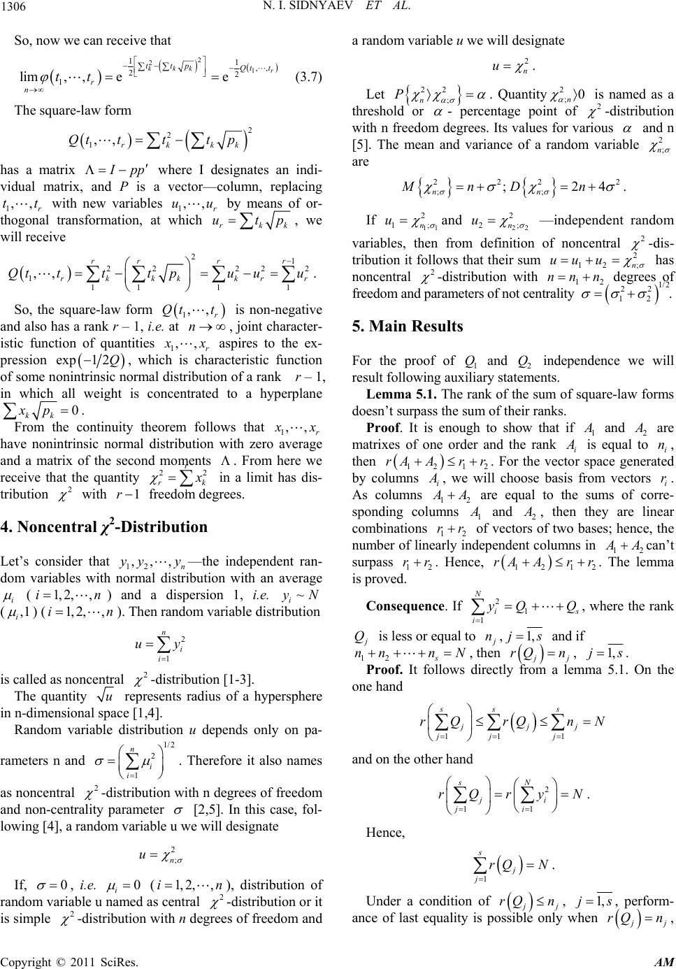

1306 N. I. SIDNYAEV ET AL.
So, now we can receive that

 
2
2
1
11,,
22
1
lim, ,ee
kkk r
ttp Qt t
r
n
tt 

 








(3.7)
The square-law form


2
2
1,, rkkk
Qtttt p


has a matrix
I
pp   where I designates an indi-
vidual matrix, and P is a vector—column, replacing
1r with new variables 1 by means of or-
thogonal transformation, at which
,,tt,,
r
uu
rk
utpk , we
will receive

21
22 22
1
111 1
,,
rrr r
rkkk kr
Qttttpu uu


 


 
2
r
.
So, the square-law form


1,, r
Qt t
n
,,
r
is non-negative
and also has a rank r – 1, i.e. at , joint character-
istic function of quantities 1
x
x aspires to the ex-
pression

exp1 2Q

, which is characteristic function
of some nonintrinsic normal distribution of a rank r – 1,
in which all weight is concentrated to a hyperplane
0
kk
xp
.
From the continuity theorem follows that 1,,
r
x
x
have nonintrinsic normal distribution with zero average
and a matrix of the second moments . From here we
receive that the quantity
1
k

22
r
r
x
  in a limit has dis-
tribution 2

with freedom degrees. 1r
4. Noncentral χ2-Distribution
Let’s consider that 12 —the independent ran-
dom variables with normal distribution with an average
,,,
n
yy y
i

() and a dispersion 1, i.e.
(
1, 2,,in~
i
yN
,1
i

) (). Then random variable distribution 1, 2,,in
2
1
n
i
i
uy


is called as noncentral 2

-distribution [1-3].
The quantity u represents radius of a hypersphere
in n-dimensional space [1,4].
Random variable distribution u depends only on pa-
rameters n and . Therefore it also names
1/2
2
1
n
i
i






2
as noncentral

-distribution with n degrees of freedom
and non-centrality parameter

[2,5]. In this case, fol-
lowing [4], a random variable u we will designate
2
; n
u



If, 0

, i.e. 0
i

 (), distribution of
random variable u named as central
1, 2,,i
2
n

-distribution or it
is simple 2

-distribution with n degrees of freedom and
a random variable u we will designate
2
n
u

.
Let


22
P
 ; n 

  . Quantity;n

is named as a
threshold or
20
 

- percentage point of 2

-distribution
with n freedom degrees. Its values for various

and n
[5]. The mean and variance of a random variable 2
;
n


are


222
;;
;2
nn
MnD n

2
4

    .
If 11
2
1; n
u

 and 22
2
2; n
u

  —independent random
variables, then from definition of noncentral 2

-dis-
tribution it follows that their sum 2
;
n 12
uu u


 has
noncentral 2

-distribution with 12 of
freedom and parameters of not centrality
nn n degrees

1/
2
2
1
2
2

  .
5. Main Results
For the proof of 1 Q and 2 independence we will
result following auxiliary statements.
Q
Lemma 5.1. The rank of the sum of square-law forms
doesn’t surpass the sum of their ranks.
Proof. It is enough to show that if 1
A
and 2
A
are
matrixes of one order and the rank i
A
is equal to i,
then
n


121
rAAr r
2


i
. For the vector space generated
by columns
A
, we will choose basis from vectors i.
As columns 1
r
2
A
A

are equal to the sums of corre-
sponding columns 1
A
and 2
A
, then they are linear
combinations 12 rr

of vectors of two bases; hence, the
number of linearly independent columns in 12
A
A

can’t
surpass 12 rr

. Hence,


rA
12
A1 r
2
r. The lemma
is proved.
Consequence. If 2
1
1
N
i
i
s
y
Q

Q


, where the rank
j
Q is less or equal to
j
n,1,js and if
1
nnn N
2s

, then

j
j
rQ n, 1,js.
Proof. It follows directly from a lemma 5.1. On the
one hand

11 1
ss s
jjj
jj j
rQrQ nN







and on the other hand
2
11
sN
ji
ji
rQ r yN









.
Hence,

1
s
j
j
rQ N


.
Under a condition of


j
j, rQ n1,j,s perform-
ance of last equality is possible only when


j
j
rQ n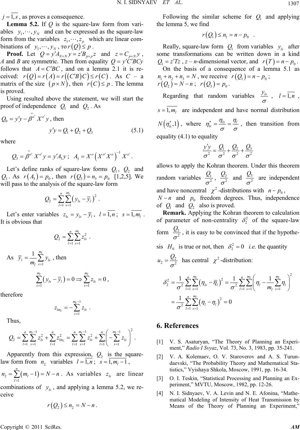

,

N. I. SIDNYAEV ET AL.
1307
1,js
, as proves a consequence.
Lemma 5.2. If Q is the square-law form from vari-
ables 1,,
N
yy and can be expressed as the square-law
form from the variables 1,,
p
zz which are linear com-
binations of 1,,
N
yy
Qy
, то .

rQ
A yz


p
B

Proof. Let NNpp
and z
pN
zCy


,
A and B are symmetric. Then from equality QyCBCy

 
follows that
A
CBC


 

rAr CBCr



pN

rC
, and on a lemma 2.1 it is re-
ceived: . As C – a
matrix of the size , then . The lemma
is proved.
 
rQ C 


p
Using resulted above the statement, we will start the
proof of independence and . As
1
Q2 Q
0
oo
QyyX 


 y
3
, then
12
yy QQQ
 (5.1)
where
33
oo
QXyyA 

 y

1
3
oooo
;
A
XXX X


.
Let’s define ranks of square-law forms 1, 2 and
3. As 0
, then
Q Q
Q

3
rA p


33
rQnp
0
1,2,5. We
will pass to the analysis of the square-law form

2
2
11
l
m
n
ls l
ls
Qy


 y.
Let’s enter variables lsls l zyy, 1,ln; 1,l
s
m.
It is obvious that
2
2
11
l
m
n
ls
ls
Qz

 .
As
1
1l
m
ll
s
l
yy
m
s , then

11
00
ll
mm
ls lls
ss
yy z

 

,
therefore
1
1
l
l
m
lm ls
s
zz




.
Thus,
2
11
22 2
2
1111111
ll
l
mm
nnnn
ls lmlsls
lsllsls
Qzzzz

  




  
1
l
m
.
Apparently from this expression, is the square-
law form from variables
2
Q
2
n1,ln; 1, 1
l
sm
,

2
1
1
n
l
l
nmN


n. As variables are linear
ls
z
combinations of , and applying a lemma 5.2, we re-
ceive
ls
y

22
rQnN n.
Following the similar scheme for and applying
the lemma 5, we find
1
Q


11
rQnnp
0

 .
Really, square-law form 1 from variables ls after
some transformations can be written down in a kind
Q y
1
QzTz


, z – n-dimensional vector, and


0
rT pn

.
On the basis of a consequence of a lemma 5.1 as
123
nnn N

, we receive ;

10
rQnp


rQN n
2

;


30
rQ p

.
Regarding that random variables ls
y

, 1,ln,
1, l
s
m are independent and have normal distribution


,1
ls
N 
, where ls l
ls




, then transition from
equality (4.1) to equality
3 12
222
Q QQ yy
2




allows to apply the Kohran theorem. Under this theorem
random variables 1
2
Q

, 2
2
Q

and 3
2
Q

are independent
and have noncentral 2

-distributions with 0 np

,
Nn

and freedom degrees. Thus, independence
of and Q also is proved.
0
p
1 2
Remark. Applying the Kohran theorem to calculation
of parameter of non-centrality
Q
2
2

of the square-law
form 2
2
Q

, it is easy to be convinced that if the hypothe-
sis 0
H
is true or not, then i.e. the quantity
2
20
 
2
2
Q
2
u

 has central 2

-distribution:


2
2
2
222
1111 1
2
2
11
11
10
ll
l
mm
nn
ls lll
lsls s
l
m
n
ll
ls
m
 



 






 

1
l
m

6. References
[1] V. S. Asaturyan, “The Theory of Planning an Experi-
ment,” Radio I Svyaz, Vol. 73, No. 3, 1983, pp. 35-241.
[2] V. A. Kolemaev, O. V. Staroverov and A. S. Turun-
daevski, “The Probability Theory and Mathematical Sta-
tistics,” Vyishaya Shkola, Moscow, 1991, pp. 16-34.
[3] O. I. Teskin, “Statistical Processing and Planning an Ex-
periment,” MVTU, Moscow, 1982, pp. 12-26.
[4] N. I. Sidnyaev, V. A. Levin and N. E. Afonina, “Mathe-
matical Modeling of Intensity of Heat Transmission by
Means of the Theory of Planning an Experiment,”

N. I. SIDNYAEV ET AL.
1308
Inzhenerno Fizicheskii Gurnal (IFG), Vol. 75, No. 2,
2002, pp. 132- 138.
[5] N. I. Sidnyaev, “The Theory of Planning Experiment and
Analysis of Statistical Data,” URight, Moscow, 2011, pp.
95-220.