Paper Menu >>
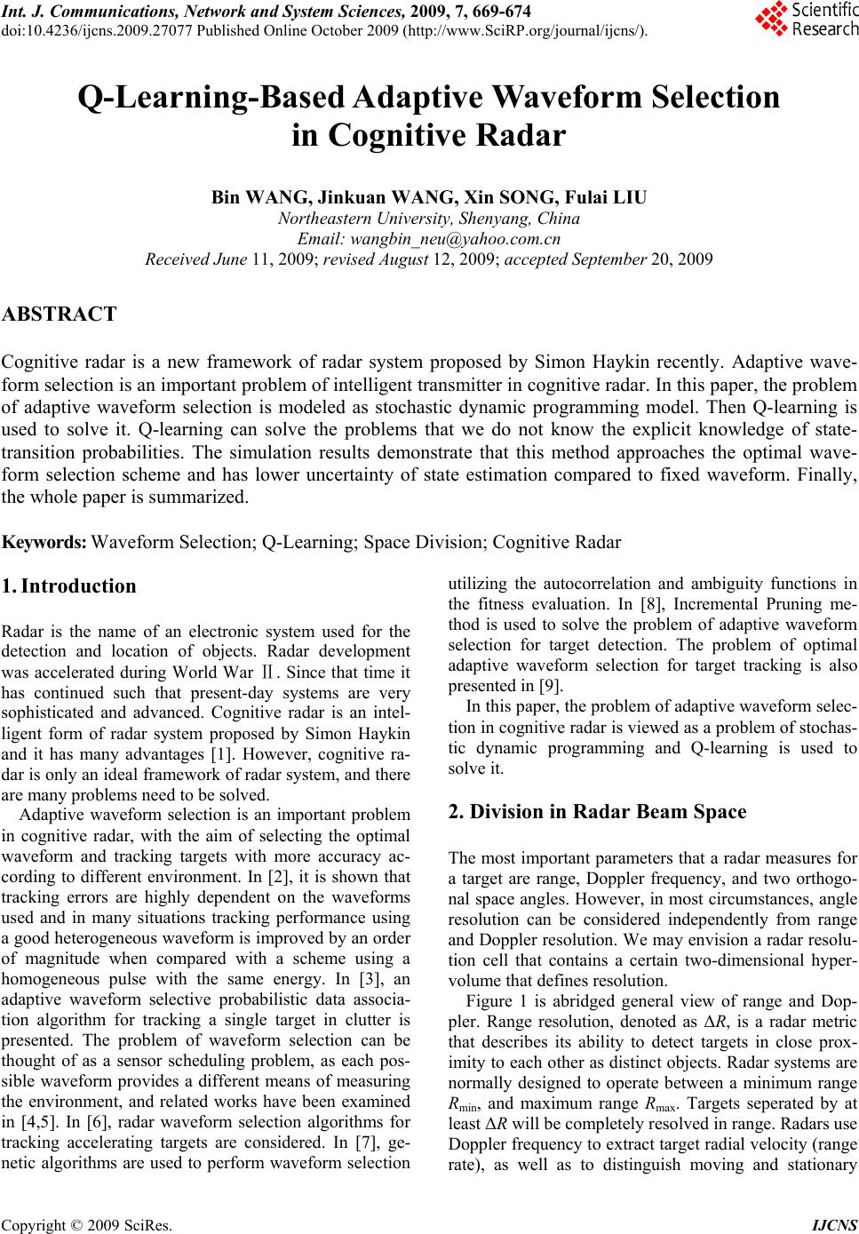
Journal Menu >>
 Int. J. Communications, Network and System Sciences, 2009, 7, 669-674 doi:10.4236/ijcns.2009.27077 Published Online October 2009 (http://www.SciRP.org/journal/ijcns/). Copyright © 2009 SciRes. IJCNS Q-Learning-Based Adaptive Waveform Selection in Cognitive Radar Bin WANG, Jinkuan WANG, Xin SONG, Fulai LIU Northeastern University, Shenyang, China Email: wangbin_neu@yahoo.com.cn Received June 11, 2009; revised August 12, 2009; accepted September 20, 2009 ABSTRACT Cognitive radar is a new framework of radar system proposed by Simon Haykin recently. Adaptive wave- form selection is an important problem of intelligent transmitter in cognitive radar. In this paper, the problem of adaptive waveform selection is modeled as stochastic dynamic programming model. Then Q-learning is used to solve it. Q-learning can solve the problems that we do not know the explicit knowledge of state- transition probabilities. The simulation results demonstrate that this method approaches the optimal wave- form selection scheme and has lower uncertainty of state estimation compared to fixed waveform. Finally, the whole paper is summarized. Keywords: Waveform Selection; Q-Learning; Space Division; Cognitive Radar 1. Introduction Radar is the name of an electronic system used for the detection and location of objects. Radar development was accelerated during World War Ⅱ. Since that time it has continued such that present-day systems are very sophisticated and advanced. Cognitive radar is an intel- ligent form of radar system proposed by Simon Haykin and it has many advantages [1]. However, cognitive ra- dar is only an ideal framework of radar system, and there are many problems need to be solved. Adaptive waveform selection is an important problem in cognitive radar, with the aim of selecting the optimal waveform and tracking targets with more accuracy ac- cording to different environment. In [2], it is shown that tracking errors are highly dependent on the waveforms used and in many situations tracking performance using a good heterogeneous waveform is improved by an order of magnitude when compared with a scheme using a homogeneous pulse with the same energy. In [3], an adaptive waveform selective probabilistic data associa- tion algorithm for tracking a single target in clutter is presented. The problem of waveform selection can be thought of as a sensor scheduling problem, as each pos- sible waveform provides a different means of measuring the environment, and related works have been examined in [4,5]. In [6], radar waveform selection algorithms for tracking accelerating targets are considered. In [7], ge- netic algorithms are used to perform waveform selection utilizing the autocorrelation and ambiguity functions in the fitness evaluation. In [8], Incremental Pruning me- thod is used to solve the problem of adaptive waveform selection for target detection. The problem of optimal adaptive waveform selection for target tracking is also presented in [9]. In this paper, the problem of adaptive waveform selec- tion in cognitive radar is viewed as a problem of stochas- tic dynamic programming and Q-learning is used to solve it. 2. Division in Radar Beam Space The most important parameters that a radar measures for a target are range, Doppler frequency, and two orthogo- nal space angles. However, in most circumstances, angle resolution can be considered independently from range and Doppler resolution. We may envision a radar resolu- tion cell that contains a certain two-dimensional hyper- volume that defines resolution. Figure 1 is abridged general view of range and Dop- pler. Range resolution, denoted as ΔR, is a radar metric that describes its ability to detect targets in close prox- imity to each other as distinct objects. Radar systems are normally designed to operate between a minimum range Rmin, and maximum range Rmax. Targets seperated by at least ΔR will be completely resolved in range. Radars use Doppler frequency to extract target radial velocity (range rate), as well as to distinguish moving and stationary 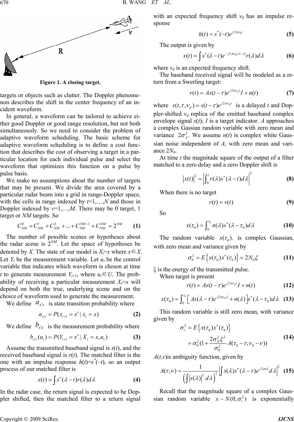 B. WANG ET AL. 670 Figure 1. A closing target. targets or objects such as clutter. The Doppler phenome- non describes the shift in the center frequency of an in- cident waveform. In general, a waveform can be tailored to achieve ei- ther good Doppler or good range resolution, but not both simultaneously. So we need to consider the problem of adaptive waveform scheduling. The basic scheme for adaptive waveform scheduling is to define a cost func- tion that describes the cost of observing a target in a par- ticular location for each individual pulse and select the waveform that optimizes this function on a pulse by pulse basis. We make no assumptions about the number of targets that may be present. We divide the area covered by a particular radar beam into a grid in range-Doppler space, with the cells in range indexed by t=1,…,N and those in Doppler indexed by v=1,…,M. There may be 0 target, 1 target or NM targets. So 01 21 ... 2 NMNM NM NM NM NMNMNM CCCC C (1) The number of possible scenes or hypotheses about the radar scene is 2NM. Let the space of hypotheses be denoted by X. The state of our model is Xt=x where x∈X. Let Yt be the measurement variable. Let ut be the control variable that indicates which waveform is chosen at time t to generate measurement Yt+1, where ut∈U. The prob- ability of receiving a particular measurement Xt=x will depend on both the true, underlying scene and on the choice of waveform used to generate the measurement. We define x x a is state transition probability where 1 (| xx tt aPxxxx ) (2) We define x x b is the measurement probability where 1 () (|,) x xttt t buPYxX xu (3) Assume the transmitted baseband signal is s(t), and the received baseband signal is r(t). The matched filter is the one with an impulse response h(t)=s*(–t), so an output process of our matched filter is ()() () x ts trd (4) In the radar case, the return signal is expected to be Dop- pler shifted, then the matched filter to a return signal with an expected frequency shift v0 has an impulse re- sponse 0 2 * ()() j t hts te (5) The output is given by 0 2() ()()( ) jt x ts terd (6) where v0 is an expected frequency shift. The baseband received signal will be modeled as a re- turn from a Swerling target: 2 ()( )() d jt rtAsteI nt (7) where 2 (, ,)()d j t d stst e 2 2A is a delayed t and Dop- pler-shifted vd replica of the emitted baseband complex envelope signal s(t); I is a target indicator. A approaches a complex Gassian random variable with zero mean and variance . We assume n(t) is complex white Gaus- sian noise independent of A, with zero mean and vari- ance 2N0. At time t the magnitude square of the output of a filter matched to a zero delay and a zero Doppler shift is 2 2 0 ()( )() t x trstd (8) When there is no target () ()rt vt (9) So 0 0 0 ()()( ) 0 x ns d (10) The random variable 0 (). x is complex Gaussian, with zero mean and variance given by 2 000 ()()2Ex xN 0 (11) ξ is the energy of the transmitted pulse. When target is present 2 ()( )() d jt rtAsteI nt (12) 02 00 0 ()()() () d j x Asen sd (13) This random variable is still zero mean, with variance given by 2 100 22 2A 00 2 0 ()() 2 (1( ,)) Ex x A 0 (14) A(t,v)is ambiguity function, given by 2 2 2 2 1 (, )( )() () j A sse d sd (15) Recall that the magnitude square of a complex Gaus- sian random variable 2 ~(0, ) i xN is exponentially Copyright © 2009 SciRes. IJCNS  B. WANG ET AL. 671 distributed, with density given by 2 2 2 2 1 ~2 i y i yx e (16) We consequently have that the probability of false alarm Pf is given by 2 0 2 2 0 1 2 2 0 2 x D fD Pedxe (17) And the probability of detection Pd by 22 2 00 2 2 0 1 2 2(1( ,)) 2 2 1 1 2 A D xA dD Pedxe 0 (18) In the case when a target is present in cell (, ) , as- suming its actual location in the cell has a uniform dis- tribution 22 2 000 2 0 2 2(1( ,)) (,) 1A aa D A d A Pe d A a a d (19) where A is the resolution cell centred on (t,v) with vol- ume |A|. 3. Q-Learning-Based Stochastic Dynamic Programming A target for which measurements are to be made will fall in a resolution cell. Another target, conceptually, does not interfere with measurements on the first if it occupies another resolution cell different from the first. Thus, conceptually, as long as each target occupies a resolution cell and the cells are all disjoint, the radar can make measurements on each target free of interference from others. Define 01 {,,..., } T uu u where T=1 is the maximum number of dwells that can be used to detect and confirm targets for a given beam. Then is a sequence of waveforms that could be used for that decision process. We can obtain different according to different en- vironment in cognitive radar. Let 0 () [(,)] T t tt tt t VX ERXu (20) where R(Xt,ut) is the reward earned when the scene Xt is observed using waveform ut and γ is discount factor. Then the aim of our problem is to find the sequence that satisfies 0 ()max[ (,)] T t tt t VXE RXu t (21) However, knowledge of the actual state is not avail- able. Using the method of [10], we can obtain that the optimal control policy that is the solution of (21) is also the solution of 0 ((0))max [( ,)] T t tt t VER ppu (22) where Pt is the conditional density of the state given the measurements and the controls and P0 is the a priori probability density of the scene. P is a sufficient statistic for the true state Xt. So we need to solve the following problem 0 max [( ,)] T t tt t ERu p (23) The refreshment formula of Pt is given by 1' t t t BAp p1LAp (24) where B is the diagonal matrix with the vector the non-zero elements and 1 is a column vector of ones. A is state transition matrix. (()) xx t bu If we wanted to solve this problem using classical dy- namic programming, we could have to find the value function using () tt Vp 11 () max((,){()| }) t tttttt tt u VRuEV pp pp (25) It can also be written in probability form 1 () max((,)(,)()) t tt tttttt u VRuPuV pP pp ppp (26) However, in radar scene, explicit knowledge of target state-transition probabilities are unknown. So directly using Bellman’s dynamic programming is very hard. The Q-leaning algorithm is a direct approximation of Bell- man’s dynamic programming, and it can solve the prob- lem that we do not know explicit knowledge of state-transition probabilities. For this reason, Q-learning is very suitable to be used in the problem of adaptive waveform selection in cognitive radar. We define a Q-factor in our problem. For a state-ac- tion pair , (,) tt up 1 (,)(,)[ (,)] tttt tttt QuPuRuV pP ppppp (27) According to (26), (27) we can derive *max ( , ) t t u VQptt u (28) The above establishes the relationship between the value function of a state and the Q-factors associated with a state. Then it should be clear that, if the Q-factors are known, one can obtain the value function of a given state from above fomula. So Q form of Bellman equation is 1 11 (,) (, )[ (, )max (,)] t tt tt ttttt u Qu PuRuQu pP p pp ppp(29) Copyright © 2009 SciRes. IJCNS  B. WANG ET AL. 672 Let us denote the ith independent sample of a random variable X by Si and the expected value by E(X). Xn is the estimate of X in the n th iteration. So 1 () lim n i i n s EX n (30) 1 n i ni s Xn (31) We can derive 111 (1 ) nnnn1n X Xs (32) where 11 1 n n (33) So 1 11 (,)[(,)max( ,)] t tttttt t u Qu ERuQu pppp (34 ) where E is the expectation operator. We could use this scheme in a simulator to estimate the same Q-factor. Using this algorithm, Equation (29) becomes: 1 11 1 11 (,)(1)(,) [(,)max (,)] t nnn tt tt nn ttttt u Qu Qu Ru Qu pp ppp (35) Obviously, we do not have the transition probabilities in it. Our Q-learning algorithm is as follows: Step 1. Initialize the Q-factors to 0. Set n=1. Step 2. For t=0,1,… T,do step 3-step 6. Step 3. Simulation action ut. Let the curren state be Pt, and the next state be Pt+1. Step 4. Find the decision using the current Q-factors: 1 arg max(,) t nn tt u uQ ptt u (36) Step 5. Update Q(Pt,ut) using the following equation: 1 11 1 11 (,)(1)(,) [(,)max (,)] t nnn tt tt nn ttttt u Qu Qu Ru Qu pp ppp (37) Step 6. Find the next state: 1' t t t BAp p1BAp (38) Step 6. Increment n. If n<N, go to step 2. Step 7. For each P t ∈P, select 11 ()arg max(,) t tt u dQ pp t u (39) The policy generated by the algorithn is . Stop. ˆ d 4. Simulation In this section, we make three experiments. In order to explain the necessity of waveform selection, we make the curve of measurement probability versus SNR of three waveforms. Curve of uncertainty of state estima- tion demonstrates validity of our proposed algorithm. We also plot the figure of Q value space versus state and waveform. We consider a simple situation. The state space is 4× 4. We consider 5 different waveforms where for each waveform u, and each hypotheses for the target x , the distribution of x is given in Table 1. The discount fac- tor γ=0.9. State transition matrix A is given by 0.960.020.01 0.04 0.01 0.93 0.03 0.04 0.02 0.03 0.95 0.02 0.01 0.020.010.9 A (40) Following the approach described in [11,12], linear form of reward function will be adopted: (,)' 1Ruppp (41) The formula E(–R) can be considered as the uncer- tainty in the state estimation. In other words, it can be considered as the tracking errors. Figure 2 is curve of measurement probability versus SNR of three waveforms. From this curve we can see that with the same SNR, different waveforms correspond to different measurement probability. Generally speaking, the waveform with wide pulse duration corresponds to high measurement probability. From this point of view, the waveform with wide pulse duration is better. How- ever, wide pulse duration means large energy of the transmitted pulse. So we should improve measurement -10 010 20 30 40 50 0 0. 1 0. 2 0. 3 0. 4 0. 5 0. 6 0. 7 0. 8 0. 9 1 SNR(dB) Meas urem ent P robabil i t y waveform 1 waveform 2 waveform 3 Figure 2. Curve of measurement probability versus SNR of three waveforms. Copyright © 2009 SciRes. IJCNS  B. WANG ET AL. 673 Table 1. Measurement probabilities for the examp le scenario. x=1 x’=1,2,3,4 x=2 x’=1,2,3,4 x=3 x’=1,2,3,4 x=4 x’=1,2,3,4 u=1 0.97,0.01 0.01,0.01 0.01,0.01 0.96,0.02 0.01,0.02, 0.01,0.96 0.96,0.01, 0.01,0.02 u=2 0.96,0.01 0.02,0.01 0.02,0.95 0.01,0.02 0.01,0.01, 0.01,0.97 0.02,0.96, 0.01,0.01 u=3 0.94,0.02 0.03,0.01 0.02,0.02 0.01,0.95 0.02,0.96, 0.01,0.97 0.01,0.02, 0.95,0.02 u=4 0.96,0.01 0.01,0.02 0.01,0.02 0.96,0.01 0.97,0.01, 0.01,0.01 0.03,0.95, 0.01,0.01 u=5 0.95,0.02 0.01,0.02 0.01,0.97 0.01,0.01 0.02,0.01 0.96,0.01 0.04,0.94 0.01,0.01 probability through changing waveforms according to different environment and make a balance between the width of pulse duration and the energy of the transmitted pulse. We can also derive measurement probabilities for the example scenario from this curve, as is shown in Ta- ble 1. Figure 3 is curve of uncertainty of state estimation. From this curve we can see that for all the cases, the un- certainty of state estimation is decreasing with time, no matter how the state is changing with time. Compared to a fixed waveform, Q-learning algorithm we proposed has lower uncertainty of state estimation. That means our algorithm will reduce uncertainty in locating targets. Meanwhile our algorithm approaches the optimal wave- form selection scheme even though explicit knowledge of state-transition probabilities is unknown. Figure 4 is the figure of Q value space versus state and waveform. Q value of different state-waveform pair can be obtained in this figure. We can see that the proposed algorithm has lower computational cost. 5. Conclusions Adaptive waveform selection is an important problem in cognitive radar and the problem of adaptive waveform 010 20304050 6070 80 90 100 0.2 0. 25 0.3 0. 35 0.4 0. 45 0.5 0. 55 time E(-R) Uncert ainty of St ate E st i m at i on Q-l earni ng opti m al s cheme fi xed waveform Figure 3. Curve of uncertainty of state estimation. 1 2 3 4 12345 0 1 2 3 4 Figure 4. Q value space versus state and waveform. scheduling can be viewed as a stochastic dynamic pro- gramming problem. In this paper, Q-learning-based waveform selecting algorithm is proposed. The advan- tages of Q-learning over fixed waveform have been shown with simulations. The Q-learning algorithm can minimize the uncertainty of state estimation compared to fixed waveform and approaches the optimal waveform selection scheme. Meanwhile, Q-learning can solve the problems in which explicit knowledge of state-transition probabilities are unknown. Reasearch on alogorithms which approach the optimal waveform selection scheme and has lower computational cost is an important problem. 6. References [1] S. Haykin, “Cognitive radar: A way of the future,” IEEE Signal Processing Magazine, Vol. 23, No. 1, pp. 30–40, 2006. [2] C. Rago, P. Willett, and Y. Bar-Shalom, “Detecting- tracking performance with combined waveforms,” IEEE Transactions on Aerospace and Electronic Systems, Vol. 34, No. 2, pp. 612–624, 1998. [3] D. J. Kershaw and R. J. Evans, “Waveform selective probabilistic data association,” IEEE Transactions on Aerospace and Electronic Systems, Vol. 33, No. 4, pp. 1180–1188, 1997. [4] Y. He and E. K. P. Chong, “Sensor scheduling for target tracking in sensor networks,” 43rd IEEE Conference on Decision and Control, Paradise, Island, Bahamas, pp. 743–748, 2004. [5] V. Krishnamurthy, “Algorithms for optimal scheduling of hidden Markov model sensors,” IEEE Trans. on Signal Processing, Vol. 50, No. 6, pp.1382–1397, 2002. [6] C. O. Savage, and B. Moran, “Waveform selection for maneuvering targets within an IMM framework,” IEEE Transactions on Aerospace and Electronic Systems, Vol. 43, No. 3, pp. 1205–1214, 2007. [7] C. T. Capraro, I. Bradaric, G. T. Capraro, and T. K. Lue, Copyright © 2009 SciRes. IJCNS  B. WANG ET AL. Copyright © 2009 SciRes. IJCNS 674 “Using genetic algorithms for radar selection,” 2008 IEEE Radar Conference, Inc., Utica, NY, pp. 1–6, May 2008. [8] B. F. La Scala and R. J. Moran Wand Evans, “Optimal adaptive waveform selection for target detection,” The International Conference on Radar, Adelaide, SA, Aus- tralia, pp. 492–496, Sept. 2003. [9] La Scala, Rezaeian, and Moran, “Optimal adaptive wave- form selection for target tracking,” International Confer- ence on Information Fusion, pp. 552–557, 2005. [10] D. Bertsekas, “Dynamic programming and optimal con- trol,” Athena Scientific, Second Edition, Vol. 1, 2001. [11] V. Krishnamurthy, “Algorithms for optimal scheduling of hidden Markov model sensors,” IEEE Transactions on Signal Processing, Vol. 50, No. 6, pp. 1382–1397, 2002. [12] W. S. Lovejoy, “Computationally feasible bounds for partially observed Markov decision processes,” Opera- tions Research, Vol. 39, No. 1, pp. 162–175, 1991. |