 Applied Mathematics, 2011, 2, 1243-1251 doi:10.4236/am.2011.210173 Published Online October 2011 (http://www.SciRP.org/journal/am) Copyright © 2011 SciRes. AM High Accuracy Arithmetic Average Discretiz ati on f or Non-Linear Two Point Boundary Value Problems with a Source Function in Integral Form Ranjan K. Mohanty, Deepika Dhall Department of Mat hematics, Faculty of Mathematical Sciences, University of Delhi, Delhi, India E-mail: rmohanty@maths.du.ac.in Received June 17, 2011; revised June 30, 2011; accepted July 6, 2011 Abstract In this article, we report the derivation of high accuracy finite difference method based on arithmetic average discretization for the solution of , 0 < x < 1, 0 < s < 1 subject to natural boundary conditions on a non-uniform mesh. The proposed variable mesh approximation is directly applicable to the integro-differential equation with singular coefficients. We need not require any special discretization to ob- tain the solution near the singular point. The convergence analysis of a difference scheme for the diffusion convection equation is briefly discussed. The presented variable mesh strategy is applicable when the inter- nal grid points of the solution space are both even and odd in number as compared to the method discussed by authors in their previous work in which the internal grid points are strictly odd in number. The advantage of using this new variable mesh strategy is highlighted computationally. 1 0 ,,, duFxuu Kxs s Keywords: Variable Mesh, Arithmetic Average Discretization, Non-Linear Integro-Differential Equation, Diffusion Equation, Simpson’s 1 3Rd Rule, Singular Coefficients, Burgers’ Equation, Maximum Absolute Errors 1. Introduction We consider the non-linear differential equation with a source function in integral form: 1 0 ,,, d,0,1uFxuuKxss xs . (1) The two point boundary conditions associated with (1) are given by: 0 0,1uu 1 (2) where 0 , 1 are finite constants. We assume that K(x, s) is a real valued function of both variables in the range 0 ≤ x, s ≤ 1. Let 1 0 ,d xKxs and ,, ,, xuuIxG xuu Then we may re-write (1) as ,, ,01uGxuu x (3) Keller [1] has given the conditions under which the differential Equation (3) together with the boundary con- ditions (2) has a unique solution. We assume that these conditions are satisfied in the problem that we are con- sidering. In addition, we assume that 60,1ux C and 4 ,0Kxs C,1. Many physical problems from fluid mechanics, fluid dynamics, elasticity, magneto-hydrodynamics, plasma dynamics, oceanography, biological model, boundary layer theory, …etc are described mathematically by non- linear integro-differential equations. Davis and Rabi- nowitz [2], Philips [3], Linz [4], Lakshmikantham and s  1244 R. K. MOHANTY ET AL. Rao [5], Atkinson [6], and Agarwal and O’Regan [7] have discussed various techniques for numerical integra- tion and methods for approximate solution of integro- differential equations and their applications to various physical models. Most of the nonlinear differential equa- tions cannot be solved analytically. So it is required to obtain efficient numerical methods. Jain et al. [8] have discussed variable mesh methods for the solution of two point nonlinear boundary value problems; however, their methods are not applicable to differential equations with singular coefficients. In recent years, Mohanty et al. ([9- 12]) have discussed a family of third order variable mesh methods for the solution of two point non-linear bound- ary value problems and obtained convergent solution for singular problems. More recently, Mohanty and Dhall [13] have proposed a three-point third order variable mesh method for the solution of non-linear integro-dif- ferential Equation (1), which is applicable only when the internal grid points of the solution region are odd in number. In this paper, we propose an efficient third order variable mesh method based on arithmetic average dis- cretization for the solution of non-linear integro-differ- ential Equation (1), which is applicable when the internal grid points of the solution region are both odd and even in number. In next section, we give mathematical details of the method. In Section 3, we discuss the application of the proposed method to an integro-differential equation with singular coefficients and study the convergence analysis. In Section 4, we give numerical results to jus- tify the utility of the proposed new strategy. Final re- marks are given in Section 5. 2. Mathematical Details of the Discretization We discretize the solution region [0,1] with the non- uniform mesh such that 01 1 01 N xx x 1N . Let 11 be the variable mesh size in x-di- rection, where . Grid points are given by 0 kkk hxx i 01k 0 1 ik k xh , . The mesh ratio is 11 1iN 10 kkk hh . When 1 k , then it reduces to the constant mesh case. The off-step points are defined by 1 22 kk k k h xx and 1 22 k k k h xx etc. Let the exact solution of u(x) at the grid point k be denoted by and u be the approximate value of . k Uuxkk k Let us construct a numerical method for evaluating the U integral 1 0 d x , where is a real-valued con- tinuous function in [0,1]. Using the derivation technique discussed in [13], we obtain a fourth order accurate integral formula based on Simpson’s 1 3rd rule (see Evans [14]). 1 1 2 1 1 d4 6 0,1, 2, k k xkk k x h xx kN , k (4) where kk , , 11kk kk xxh 1 1 11 22 2 k k kk h xx , etc. Then on the variable mesh the value of the integral 1 12 01 1 0 1 11 02 ddd 4 6 N N x xx xx x Nkkk k k d xxxxxx h x (5) can be found by the repeated application of (4). Now we discuss the third order numerical method based on arithmetic average discretization for the differential Equation (3). At the grid point k , we denote ,, kkkk k UGxUU G (say), and , kk kk x GG uu . Using Taylor expansion, from (3), we obtain 11 2 5 11 22 1 1, 32 1 kkkkk k kk kk kk k UUU hGGGO k h (6) We need the following approximations: 11 2 1 2kk k UUU , (7a) 11 2 1 2kk k UUU , (7b) 11 2 1 kk kkk UU h U , (7c) 1 2 1 kk kk UUU h 1 , (7d) Copyright © 2011 SciRes. AM  R. K. MOHANTY ET AL. Copyright © 2011 SciRes. AM 1245 22 11 11 1 kkkk kkk UUU h 22 3 11 22 3, 24 1 kk kk kkk kk k h GGUU Oh (9a) kk U, (7e) and let 2 3 11 22 3, 24 1 kkkkkk kk k h GGUU Oh (9b) 1 111 2 222 ,, k kkk GGxUU . (8) From (9a) and (9b), it follows that It is then easy to see that 2 23 11 22 2113 3, 224 IV kk kkkkkkkkk kk kk hh GGUUU UUOh 1 (10a) 2 23 11 22 1133 224 IV kk kkkkkkkkk k kk hh GGUU UUOh ,1 (10b) 23 2, kk kkkk UU ahUOh Now, let 1 , (12a) 2 11 22 kk k kk UUahGG , (11a) 2 3 31 , 6 1 k kkkkkk k h UUb UOh (12b) 11 22 kkk kk UUbhG G , (11b) Further, we define ,, k kkk GGxUU (13) where “a” and “b” are parameters to be determined. With the help of (10a) and (10b), from (11a) and (11b), we obtain and with the help of (12a) and (12b), it follows that 2 23 231 6 k kk kkkkkkkkk h GG ahUbUOh ,1 (14) Then at each internal grid point xk, the differential Equation (3) is discretized by 2 1111 22 1 1, 32 k kk kkkkkkk k kk h UUUG GGTk 11 N (15) where 5 kk TOh, provided 1 k . Now with the help of the approximations (9a), (9b) and (14), from (6) and (15), we obtain the local trunca- tion error 4 22 1318 161, 72 k kkk kkkkkkkkkkk h TaUbU 5 1 Oh (16) The proposed numerical method (15) to be of 3 k Oh , the coefficient of in (16) must be zero and we obtain the values of parameters 4 k htial equation 1 2 2 0 ,d, 0, 1 du du rBrufrKrs dr dr rs s (17) 22 11 ,, 86(1 kk kk k ab ) where 2 ,ArBr rr and the local truncation error given by (16) becomes 5 kk TOh, 1 k . . For = 1 or 2, the equation above represents cylindrical or spherical prob- lem, respectively. Replacing the variable x by r and ap- plying the formula (15) to the integro-differential equa- 3. Application to Singular Problems Consider the linear second order model integro-different- tion (17), we obtain  1246 R. K. MOHANTY ET AL. 2 1111111 1 22222 2 111111 22222 2 13 10,11 2 kk kkk kkk kkkkk k kkkkkkkk kkkkk k h UUU AUBUfI UBUfI AUBUfITk N (18) where ,,, kkkkkkkk UurAArBBrffr , 1 12 01 1 0 ,d ,d N N r rr kk kk rr r IrKrssKrss , 22 11111 111111 1 22222 222222 2 1 8 kkk kk kkkkk kkkkkkk h UUAU BUf IAU BUf I , 2 11 1111 111111 22 222222 2222 1 61 kkk kk kkkkk kkkkkk k k h UUAU BUf IAU BUf I , nd eme (18) is directly applicable to sin- gu he scheme (18), we use the fol- lo a 5 kk TOh. te that the schNo lar problem (17) and do not require any fictitious points outside the solution region to compute the scheme. The scheme is also applicable when the internal grid points of the solution region are both even and odd in number as compared to the scheme discussed by Mo- hanty and Dhall [13] in which the internal grid points are strictly odd in number. For convergence of t wing approximations: 22 3 1 228 kk kk kk k k hh k IIIO h , (19a) 2 3 1 228 kk kkk k hh k IIIOh , (19b) 22 3 1 228 kk kk kk k k hh k AAAO h , (19c) 2 3 1 228 kk kkk k hh k AAAOh . (19d) Similarly, we can define the approximations for 1 2 k B and 1 2 k f, where ,, ,, ,e kkkk kk dd AArBBr dr dr dK ffrKrs dr r tc and 1 12 01 1 0 ,d ,d, N N kk k r rr k rr r d IIrKrss dr rs s 1 12 01 1 2 2 0 ,d ,d. N N kkk r rr k rr r d IrK rs s dr rs s Using the approximations (19) in (18), neglecting high order terms and simplifying we get the modified scheme in compact form 1 1 1 10 kkkk k kkk k k ub UdiagU sup UT (20) where 2 2 2 22 23 6328 62 12 72 11 , 48 kkkkk k kkkkk kk k kk kkkkk kkk k kk kkkkk hhhh subAAAA hh BB Ah AhAB ABh Copyright © 2011 SciRes. AM  R. K. MOHANTY ET AL. 1247 222 22 22 23 2 1 1 11 11 6643 48 1111 12, 362 48 kkkkk kkkkkkkkkkk kkkk kk kkkkkkkkkk kkk kkk hB hh hhB diaghAAAB Ah Bh Bh AA kkk Bh 22 22 222 3 632 862 11 2, 72 48 kkk kkkkkkkk kkk kkk k kk kkkkkkkk kkkkk hh hhhh supAAAABB 1 hA AABh Bh 22 2 22 2 1 13 64 11 1, 12 4 kkkk kkk kkk kkkk kk kkkk Bh hfI Ah hf Ihf I kkk and Ine boundary values 5. kk TOh corporating th00 U , 11N U , can be writ-the difference Equation (20) in ma ten as (21) where trix form k h 0DPU T ,1, 1 kk D are tri-diagonal matrices of order and P = [subk, diagk, supk] N and 1102 11 ,,,,1 T NNN sub sup , T 12 ,,, N UU U, 12 ,, k hTT 0, 0,, 0T 0 are vectors. U ,T TT 12 ,,, T N uu u uU which satisfies N and Let 0DPu (22) Let kkk euU nce of 12 ,,e U btracting (21) f be the discretization error (in the abse round of errors) at the grid point rk and be the error vector. ), we obtain the error equa- tion ,T N eEu Surom (22 e k hDPET (23) Let 1k G , 2k G , 3k G , 1k BH, 2k BH , 3k B 3, H1, H2 and HH, where G1, G2, G3 are some positive constants. If pi, j be the (i, j)th-element of P, then 2 3 , 111, kkk hGOhkN (24a) 2 ,1 11 1 12 66 k kk k k h pG 2 2 1 k k hGH 2 23 ,112 11 1 12 , 21 66 kkk kkk kk h pGhGHGOhk Thus for suffic, the matrix (D r- educible (see Voung [16]). , N (24b) kk h iently small hk arga [15] and Y + P) is i r Let Sk be the sum of elements of the kth-row of (D + P), then 2 2 23 1 12 23, 666 kk kk kkkkkkkkk k hh SAhABAO 1 hk (25a) 2 2 22 1 112 32, 3 66 6 kk kk kkkkkkkkk kk hh SAhA BAOhkN , (25b) Copyright © 2011 SciRes. AM  1248 R. K. MOHANTY ET AL. 3 1,211. 2 k kk k kk h SBOhkN (25c) 2 Let 1*1 min k kN GA , 11 max k kN GA , 1*1 min k kN B , 11 max k kN B , then 0 < G1* ≤ G1 ≤ and 0 < H1* ≤ H1 ≤ 1 G 1 . It is straightforward to show that for sufficiently small hk, (D + P) is Monotone (see Varga [15] and Young [16]). Hence (D + P)–1 exists and (D + P)–1 ≥ 0. From error Equation (23), we have 1 k h EDPT for sufficiently small hk, it is easy to show that (26) Thus 2 1* 23, 1 6 k k k hHk , (27a) k S 2 1* 32 , 6 k kkk SH kN , (27b) h 2 1,21 k h SHkN 1* 2 kk k1. (27c) Since 1 ,0 ik DP and , 1ik k DP . 1 k S, 1 N 11iN, hence 1 2 , 1* 16 ,1 23 ik kkkk k SHh DP (28a) 1 2 , 1* 16 , 32 ik kkkk kN SHh DP Further, (28b) 1N1 2 21* 12 , min 1 11 kkkk kN S , 21 ik k h iN DP (29 For any matrix M, we define ) , 1 ik k m , 1 max N iN M where is the (i, k)th-element of M and ,ik m 1 max ki iN hT T. With the help of (28a), (28b), (29), from (26), we ob- tain 5 2 1* 3 61 1 1 23 3132k kkk kk k Oh Hh Oh E (30 This establishes the third order convergence of the method (20). merical Results In this section, we consider another ne method for the solution of non-linear in Equation (1) as ) 4. Nu w variable mesh tegro-differential 11 2 11 22 23 3 kk 2 4 11 1 12 2 12 2, 11 kkkkk kk kk k kk k UUU hFF h 22 23 3 kk k IOh N (31) where k 111 2 222 ,, k kkk FFxUU , 1 1111 ,,FFxUU , 2222 kkkk and 1 ,d,11 . kkk 0s IxKxs skN The approximations associated with 1 2 k defined by (7a)-(7d). The order of accuracy of the method (31) is of are already 2 k Oh we replace the i . For evaluating the integral associated with (31), ntegral by the trapezoidal rule (see Evans [14]). 1 12 01 1 0 1 1 0 ddd 2 N N x xx xx x Nkkk k d xxxxxx h x (32) In this section, we have solved two benchmark prob- lems using the proposed method described by equation (15) and compared our results with those obtained by using the variable mesh method discussed by Mohanty and Dhall [13] only for the cases wheinternal grid points are odd in number. We have also puted our ts using uniform mesh (when n com resul 1 k y be ob ) for all values e boundary conditions matained using the exact solution as a test procedure. The linear difference equation has been solved using a tri-diagonlver, whereas non-linear difference equations have been solved using the Newton-Raphson method (see Kelly [17] and of N. Th al so Copyright © 2011 SciRes. AM  R. K. MOHANTY ET AL. 1249 Ev aph the iterations were stopped when absolute error tolerance 1, ans [18]). While using the Newton-Rson method, ≤10–12 was achieved. The unit interval [0,1] in the space-direction is divided into (N + 1) points with 0 01 1NN xxxx where 1kkk hxx and 10,1,2,,. kkk hh kN We may write 10 1110 1111212 1NNNNN NN N xxxx xxxx hh hh 1 1. (33) For simplicity, we consider k (a constant), k = 1, (N + 2), we can compute the value of h1 from (34). This is the first mesh spacing on the left of the boundary and the remaining mesh is determined by 2, , N, then from (33) we have 11 1. 1N h (34) By prescribing the total number of mesh points to be 1kk hh , oose the va k = 1, 2, N. For variable mesh, we chlues of , 1.2. All computations were carrg dou- ble precision arithmetic. ied out usin Example 4.1 1 2 22 dd 2 d d uu urr rr rr 0 2 4e ed,01, s rrs rsr polar coordinates) (35) (Linear equation in The exact solution is given by 2 r ur re . The maximum absolute errors are tabulated in Table 1 for various values of N. Example 4.2 2 22 dd d 2 d uu u uu r2 4 e dd r r r rr r r 1 3 0 2 2e2ed,01, s rrs rrrs r (Model Burger’s equation in polar coordinates) (36) The exact solution is given by 2e r urr . The maxi- mum absolute errors are tabulated in Table 2 for various valuesf N. o 5. Final Remarks s umerical methods of accuracy of based on ar e discretizations for tlution of the non-linear integro-differential Equation (1). Mohanty and Dhall [13] have developed a thi esh method based on Numerov type ich is only applicable to the solution space having odd nuoposed va ebut applicable to the lution space having both odd and even number of in- ternal grid points. In addition, the proposed methods are directly applicable to singular problems and we do not require any fictitious points near the boundaries to in- and appli tabulate either in increasing or in de- creasing order. So it is not possible to estimate the order of convergence of the proposed method. Order of con- vergence can be estimated for unifom mesh using the formula U new n ing three variable mesh points, we have discussed a 3 k Oh he soithmetic averagr rd order variable discretization, m wh mber of grid points. Although the prriable sh method involve more algebra, m so corporate the singular point. The numerical results indi- cate that the proposed method is computationally nearly equal to the method discussed in [13]cable to the solution space with all internal grid points. We have d maximum absolute errors for different mesh sizes. Our mesh sizes are 12 12hh1 h2 h the maximum absolute errors for two grid mesh widths log logee hh, where and are e e 1 h and 2 h, respectively. For ex: in Table 2, let us con- sider the case 1 , 0.01 , N = 30 and N = 60, i.e. 1 1 30 hh (say) and 2 1 60 hh (say) and the corre- sponding maximum absolute errors are 0.3116 (–8) and 0.1978 (–9), respectively. Using the above formula the Copyright © 2011 SciRes. AM 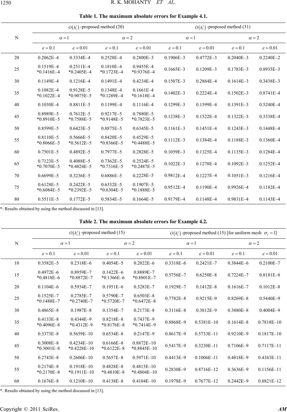 R. K. MOHANTY ET AL. 1250 Table 1. The maximum absolute errors for Example 4.1. 3 k Oh -proposed method (20) 2 k Oh -proposed method (31) 1 2 1 2 N 0.1 0.01 0.1 0.01 0.1 0.01 0.1 0.01 20 0.2062E–4 0.3334E–4 0.2528E–4 0.2800E–3 0.1906E–3 0.4772E–3 0.2040E–3 0.2240E–2 25 0.1519E–4 0.2511E–4 5E–4 0.1810E–4 *0.1 0.9455E–4 6E 34E *0.1022E–4 *0.9075E–5 *0.1289E–4*0.1618E 4 0.8811E–5 0.1199E–4 0.1116E 0.8989E–5 0.7612E–5 0.9217E–5 0.7880E 23E 0.88745E 29E 88E 112E–3 0.1384E–4 E 28E 24E 7E 78E–4 28E–5 0.981E–4 0.1 888E 64E–5 0.9179E–4 0.1148E–4 0.9831E–4 0.1143E–4 *0.1416E–4 *0.240723E–4*0.937–40.1665E–3 0.1209E–3 0.1783E–3 0.8935E–3 –4 0.1507E–3 0.2864E–4 0.1614E–3 0.3438E–3 –4 –4 0.1402E–3 0.2224E–4 0.1502E–3 0.8741E–4 –4 0.1299E–3 0.1599E–4 0.1391E–3 0.5240E–4 45 *0.8910E–5 *0.7588E–5 *0.9148E–5 –5 *0.78 –50.1238E–3 0.1522E–4 0.1322E–3 0.3338E–4 50 0.8599E–5 0.6423E–5 5E–5 0.63–5 0.1161E–3 0.1451E–4 0.1243E–3 0.1448E–4 55 0.8110E–5 *0.8066E–5 0.5666E–5 *0.5612E–5 0.8420E–5 *0.8366E–5 0.45 *0.44 60 0.7501E–5 0.4892E–5 0.7977E–5 0.28 65 0.7123E–5 *0.7070E–5 0.4088E–5 *0.4024E–5 0.7362E–5 *0.7316E–5 0.25 *0.248 70 0.6699E–5 0.3236E–5 0.6886E–5 0.22 75 0.6128E–5 *0.6084E–5 0.2422E–5 *0.2392E–5 0.6332E–5 *0.6304E–5 0.1907E *0.1 80 0.5511E–5 0.1772E–5 0.5834E–5 0.16 30 0.1149E–4 0.1216E–4 0.1491E–4 0.42 35 0.1082E–4 0.9128E–5 0.1348E–4 0.1661E 40 0.1030E– –5 –5 0.10.1188E–3 0.1360–4 –5 0.1059E–3 0.1325E–4 0.1135E–3 0.1284E–4 –5 –5 0.1022E–3 0.120.1092E–3 0.1252E–4 2E–4 0.1227051E–3 0.1216E–4 –5 –5 0.9512E–4 0.1190E–4 0.9926E–4 0.1182E–4 *: Results obtained by using the method discussed in [13]. m absolute errors for Example 4.2Table 2. The maximu. 3 k h- O 2 k Oh - proposed method (15) proposed method (15) [for uniform mesh 1 k ] 1 2 1 2 N 0.1 0.01 0.1 0.01 0.1 0.01 0.1 0.01 10 0.3582E–5 0.2318E–6 0.4054E–50.2022E–6 0.3318E–6 0.2421E–7 0.3844E–6 0.2100E–7 15 0.4972E–6 *0.4818E–6 0.8959E–7 *0.8872E–7 0.1422E–6 *0.1366E–6 0.8889E–7 *0.8801E–7 0.5756E–7 0.6250E–8 0.7224E–7 0.8181E–8 20 0.1104E–6 0.5934E–7 0.1951E–60.3283E–7 0.1929E–7 0.1412E–8 0.1616E–7 0.1012E–8 25 0.1525E–7 *0.1488E–7 0.2785E–7 *0.2740E–7 0.5790E–7 *0.5720E–7 0.6503E–8 *0.6472E–8 0.7782E–8 0.9215E–9 0.8269E–8 0.5440E–9 30 0.4865E–8 0.1987E–8 0.1354E–70.2173E–8 0.3116E–8 0.3812E–9 0.3880E–8 0.4004E–9 35 0.4133E–8 *0.4096E–8 0.4344E–9 *0.4312E–9 0.8218E–8 *0.8176E–8 0.7437E–9 *0.7414E–9 0.8868E–9 0.5381E–10 0.1614E–8 0.7818E–10 40 0.3373E–8 0.5659E–100.6534E–80.2147E–9 0.8617E–9 0.5733E–11 0.9210E–9 0.1817E–10 45 0.3008E–8 *0.3001E–8 0.4234E–10 *0.4228E–10 0.6166E–8 *0.6122E–8 0.8872E–10 *0.8845E–10 0.5417E–9 0.3230E–11 0.7106E–9 0.7117E–11 50 0.2743E–8 0.2606E–100.5657E–80.5971E–10 0.4413E–9 0.1006E–11 0.4818E–9 0.4343E–11 55 0.2174E–8 *0.2170E–8 0.1918E–10 *0.1911E–10 0.4828E–8 *0.4810E–8 0.4815E–10 *0.4804E–10 0.2830E–9 0.8716E–12 0.3636E–9 0.1156E–11 60 0.1676E–8 0.1210E–100.4138E–80.4104E–10 0.1978E–9 0.7677E–12 0.2442E–9 0.8821E–12 *: Results obtained byethod13] using the m discussed in [. Copyright © 2011 SciRes. AM  R. K. MOHANTY ET AL. 1251 order coofn ed n other cases, e found that the order of the convergence of the method for uniform mesh case is nearly e 6. Acknowledgements The authors thank the anonymous reviewers for constructive suggestions, which greatly improved the standf the This researcporhety Delhider rnt 01 423. 7. Rrence [1] . Kelleal Twoun e Plain, [2] P. J. Davibith ri tion,ionPr Yor 1970. [3] . Phil Ih for Solving In puter Jl. 10, . .3.2 of thenvergence method cabe estimatas 3.97 which is nearly equal to 4.0. Similarly i w qual to four. r thei ard opaper. h was supted by “T Universiof ” unesearch graNo. Dean (R)/R & D/21/ efes H. Br, “NumericMethods foro Point Bd- ary Valuroblems”, Bsdell, Londo1968. s and P. Ranowitz, “Meod of Numecal Integra” 2nd Edit, Academic ess, New k, G. Mlips, “Analysis of Numericalterative Metods tegral and In ournal, Vo tegro-Differential Eq 3, No. 3, 197 uations,” pp. 297-300Com doi:10.1093/comjnl/13 97 [4] P. Linz, “Ar S in ro-Dif qua N 44. Method foApproximate olution of Lear Integferential Etions,” SIAMJournal onu- merical Analysis, Vol. 11, No. 1, 1974, pp. 137-1 doi:10.1137/0711014 [5] V. Lakshmikantham and M. R. M. Rao, “Theory of Inte- gro-Differential Equations,” Gordon and Breach, London, 1995. [6] K. E. Atkinson, “The Numerical Solution of Integral Equations of the Second Kind,” Cambridge University Press, Cambridge, 1997. doi:10.1017/CBO9780511626340 MApp nic eer , 1984, pp. 273-286. doi:10.1016/0045-7825(84)90009-4 [7] R. P. Agarwal and D. O’Regan, “Integral and Integro- Differential Equations: Theory, Method and Applica- tions,” Gordon and Breach, London, 2000. [8] M. K. Jain, S. R. K. Iyenger and G. S. Subramanyam, “Variable Mesh Methods for the Numerical Solution of Two Point Singular Perturbation Problems,” Computer ethods in lied Mechas and Engining, Vol. 42 [9] R. K. Mohanty, “A Family of Variable Mesh Methods for dr) and the Solution of Nonlinear s with Singularity,” Journal atics ol. 182, No. 1, 2005, pp. 173-187. doi:10.1016/j.cam.2004.11.045 the Estimates of (du/ Two Point Boundary Value Problem of Computational and Applied Mathem, V [10] R. K. Mohanty and N. Khosla, “A Third Order Accurate Variable Mesh TAGE Iterative Mthe Num STNoguly Va em Mathematics, V26 doi:10.1080/002 ethod for nlinear Sin erical ar Boundarolution of wo Point lue Probls,” International Journal o ol. 82, No. 10 f Computer 1-1273. , 2005, pp. 1 07160500113504 [11] R. K. Mohanty and N. Khosla, “Application of TAGE IEffi Or- tic Average Variable Mesh Discretization for Two Point NBoue Ap - matics and Computations, Vol. 172, No. 1, 2006, pp. 1:1 .2 terative Algorithms to an cient Thirdder Arithme on-Linear undary ValProblems,”plied Mathe 48-162. doi 0.1016/j.amc 005.01.134 [12] R ntof Non-Uniforme Petisor . K. Moha oint Arithm y, “A Class ic Average D Mesh Thre cretization f (, ,yfxy)y and the esd Mathematics and Computations, No. pdoi:10.1016/j.am 71 timates of , Vol. 183 y,” Applie 1, 2006, p. 477-485. c.2006.05.0 [13] R. K VshcatE Iterative Methody Value Problemgetioal Form,” Applied Mathematics and Computations, Vol. 215, . Mohanty and ariable Me D. Dhal Discretization l, “Third Order and Appli Accurate ion of TAG for the Non-Lin s with Homo ear Two-Point B neous Func oundar ns in Integr 2009, pp. 2024-2034. doi:10.1016/j.amc.2009.07.046 [14] G. Evans, “Practical Numerical Integration,” John Wiley & Sons, New York, 1993. [15] R. S. Varga, “Matrix Iterative Analysis,” Springer-Verlag, Berlin, 2000. doi:10.1007/978-3-642-05156-2 [16] D. M. Young, “Iterative Solution of Large Linear Sys- tems,” Dover Publication, New York, 2003. or Solving Nonlinear blems,” International [17] C. T. Kelly, “Iterative Methods for Linear and Non-linear equations,” SIAM Publication, Philadelphia, 1995. [18] D. J. Evans, “Iterative Methods f Two Point Boundary Value Pro Journal of Computer Mathematics, Vol. 72, No. 3, 1999, pp. 395-401. doi:10.1080/00207169908804862 Copyright © 2011 SciRes. AM
|