Paper Menu >>
Journal Menu >>
 Applied Mathematics, 2011, 2, 1221-1224 doi:10.4236/am.2011.210170 Published Online October 2011 (http://www.SciRP.org/journal/am) Copyright © 2011 SciRes. AM On Canard Homoclinic of a Liénard Perturbation System Makoto Hayashi Department of Mathematics, College of Science and Technology, Nihon University, Chiba, Japan E-mail: mhayashi@penta.ge.cst.nihon-u.ac.jp Received June 8, 2011; revised August 17, 2011; accepted August 24, 2011 Abstract The classification on the orbits of some Liénard perturbation system with several parameters, which is rela- tion to the example in [1] or [2], is discussed. The conditions for the parameters in order that the system has a unique limit cycle, homoclinic orbits, canards or the unique equilibrium point is globally asymptotic stable are given. The methods in our previous papers are used for the proofs. Keywords: Liénard System, Canards, Limit Cycles, Homoclinic Orbits, Global Asymptotic Stability 1. Introduction We shall consider the Liénard perturbation system 32 3 32 , x x xy ykxa (P1) where a, , and k are positive real numbers. System (P1) has a unique equilibrium point at 33 x a and the uniqueness of solutions of initial value problems for the system is guaranteed. In [1], it has been given that the unique equilibrium point of System (P1) for the case a = 0 and 1 is a global attractor but unstable. In [2], when 1 and a = 0, the result that System (P1) has the special orbit called “a Canard Homoclinic” has been announced by the method of non standard. Our aim is to classify the orbits of System (P1) completely by the values of the parameters. Thus, we improve the results of the papers [1,2]. Our main results are the following Theorem 1.1. System (P1) has homoclinic orbits lo- cally if and only if (a = 0 and 8k ). Then the system has no limit cycles. Theorem 1.2. System (P1) has a unique limit cycle if and only if 01a. Specially, if and a are sufficiently small, the orbit is called “a Canard Limit Cycle”. Theorem 1.3. The unique equilibrium point (0, 0) for System (P1) is globally asymptotic stable if and only if one of the following 0a or 0a and 8k or 1a is satisfied. In Section 2, we shall see that System (P1) is trans- formed to a usual Liénard system (see System (P3)) with the unique equilibrium point at the origin. In Section 3, the existence of the homoclinic orbit of the system will be discussed by using the method in [3]. In virtue of this result, the interesting fact that both the limit cycle and the homoclinic orbit of the system cannot coexist is giv- en. If a > 0, a and are sufficiently small, it has been well-known b y E. Benoît ([4]) that System (P3) has the orbit called “a Canard”. The orbit changes to the ho- moclinic orbit for the system as a = 0. So the orbit has been called “a Canard Homoclinic” ([2]). In Section 4, the fact that the system has at most one limit cycle will be proved by using the method of [5]. When 01a , a and are sufficiently small, the orbit‘Canard’ spi- rals to a unique limit cycle of the system. We call the orbit “a Canard Limit Cycle”. In Section 5, it shall be seen from the facts of Section 3 and Section 4 that the unique equilibrium point for the system with the pa- rameters in Theorem 1.3 is globally asymptotic stable. Finally, a phase portrait of System (P1) with respect to Theorem 1.1 will be presented in Section 6. 2. Transformation to a Liénard System By using the transformation tt , x x and  M. HAYASHI Copyright © 2011 SciRes. AM 1222 yy for System (P1), the system is changed to the following 32 3 32 . x x xy ykxa (P2) Moreover, using the transformation x x and 2 2yy for satisfying the equation 30a , System (P2) is transformed to the system 2 22 23216 1 6 33. xy xxx ykxx x (P3) System (P3) has a unique equilibrium poin t (0, 0) and the uniqueness of solutions of initial value problems is also guaranteed. We set 2 ()232161 , 6 Fxx xx 22 g33xkxxx and 0d. x Gx g From the value of , the graph of the characteristic curve y Fx is divided into four cases; 1.. 1,ie a 10..01,ie a 0.. 0ie a and 0.. 0.ie a We will note that the situation of the graph is deeply concerned in the qualitativ e prop erty of the orbits. 3. Proof of Theorem 1.1 In System (P3), a trajectory is said to be a homoclinic orbit if its - and - limit sets are the origin. If Sys- tem (P3) has a homoclinic orbit, 0Fx (or 0Fx ) in the neighborhood of the origin is necessary. Thus we have the assumption 0.. 0iea in this section. Consider a function x with the condition [C1] 1,00and 0CxFxx for 0.x The following resul t has been given in [3] . Lemma 3.1. System (P3) with 0 has homoclinic orbits if and only if there exists a function x with [C1] such that [C2] 0Fx x and 0 x Fx xgx for 0.x As the supplement function in the above lemma, take 2 x rx with 8k and 2 48rk . Then we have 22312 0 6 Fxxx xr and 323123 0 3 xFxx gx xrx rrk for 03122.xr Thus, we see that the conditions [C1] and [C2] are satis- fied. Hence System (P3) has (l ocal) homoclinic orbits. Moreover, the following is known by the Corollary 3 in [3]. Lemma 3.2. If the conditions [C1] and [C2] hold for 1 xx and 10,x then System (P3) with 0 has homoclinic orbits locally, but no limit cycles. Taking 1 x in the proof of Lemma 3.1, we see that the above lemma holds. Therefore, the proof of Theorem 1.1 is completed now. When a > 0, a and are sufficiently small, it has been well-known from [4] that System (P3) has the orbit called “a Canard”. The orbit “Canard” changes to the mentioned homoclinic orbit above as a = 0. So the orbit has been called “a Canard Homoclinic” by [2]. Thus, we see that there exists a canard hom oclinic in System (P1). 4. Proof of Theorem 1.2 We shall assume the condition 10 (i.e. 01a ). Then we can easily check that System (P3) has at least one limit cycle. In facts, the unique equilibrium point (0, 0) is a unstable focus by (0) 0F and the all orbits are uniformly ultimately bounded (for the details see [6]). Thus, by the well-known Poincaré-Bendixson theorem, the system has a limit cycle (for instance see [7]). The following is a useful method ([5]) in order to guarantee that a Liénard system has at most one limit cycle. Lemma 4.1. If there exists a constant 0m such that 0FxGx mFxgx for 0,x System (P3) has at most one limit cycle. We have 2;, , 12 k FxGx mFxgxxxm where  M. HAYASHI Copyright © 2011 SciRes. AM 1223 43 2 2 3 ;,3436 124 1 1531 221 685343 18 121 . x mmx mx mx mx m Let 12m and 14 in ;,xm . Then we have 2 2 113 3 ;,0 0. 244 8 xxx x Thus, we see from Lemma 4.1 that System (P3) has at most one limit cycle. So we conclude that System (P3) has a unique limit cycle if –1 < α < 0. Conversely, suppose that System (P3) has a limit cycle. Then if System (P3) doesn’t satisfy the condition –1 < α < 0, this contradicts to the existence of the limit cycle by Theorem 1.1 and the proof of Theorem 1.3 (see Section 5). Therefore, the proof of Theorem 1.2 is completed now. In virtue of E. Benoît ([4]), if a > 0, a and are sufficiently small, then System (P3) has the orbit called “a Canard”. Then the orbit “Canard” spirals to a unique limit cycle of System (P3). So we call the special limit cycle “a Canard Limit Cycle”. 5. Proof of Theorem 1.3 In this section, we shall assume the condition 1 or 0 (i.e. 0a or 1a). The following is a powerful method (see [8]) to prove the non-existence of non-trivial closed orbits of a Liénard system. Lemma 5.1. If the curve , F xGx has no in- tersecting points with itself, then System (P3) has no non- trivial closed orbits. From the situation of the graph , y Fx we shall prove the theorem by dividing into four cases; i) 012, ii) 12 , iii) 32 1, iv) 32. First, we shall discuss the case i). The discussion is similar to the method shown in [9]. Let 1, 2 i pi be the solutions of the equation 0Fx and 12 0.pp Now we consider the equation Fx F for 11.p This equation has two roots other than .x Let 11 uu and 22 uu denote these roots. Then we have 12 1up and 2 012.u From a property of the curve , F xGx , we shall show that, if 12 F uFu for 11,p then 21 0.GuGu From 12 F uFu we have 22 1122 12 2321610.uuuuuu Thus we get 22 21 211212 222 112212 () 4 46. k GuGuuuu uuu uuuuuu Since 1 u and 2 u are solutions of the equation ,Fx F we have 12 32 1 2 uu and 12 31.uu Thus we get 22 2 12 9 33 . 4 uu By substituting 12 uu and 22 12 uu to 21 Gu Gu, we have 21 21 , 4 k GuGuuu L where 32 332 94278.L Then we have 0L for all and 0L 27 80 . Thus we get 0L for 0. From these facts and 21 0uu , if 0 , we conclude that 21 GuGu G for 11p . Namely, the curve , F xGx has no intersecting points with itself. This means that System (P3) with 012 has no non-trivial closed orbits. Similarly we can check that 0L for 12 and 0L for 1. Thus we have 21 0Gu Gu for 12 or 1. Therefore, we conclude that System (P3) also has no non-trivial closed orbits for the another cases ii), iii) and iv). We say that the equilibrium point 0,0E is globally asymptotically stable if E is stable and every orbit of System (P3) tends to E. We will see the global asymp- totic stability of E from the following conditions: [i] all orbits of System (P3) are bounded in the future, [ii] System (P3) has no non-trivial closed orbits, [iii] System (P3) has no homoclinic orbits, [iv] E is asymptotic stable. The condition [i], [ii] or [iii] has been checked in Sec- tion 3, Section 4 or the mentioned fact above. So we shall check the condition [iv]. Suppose that E is not stable. Then, by checking the direction of the vector ,yFx gx for System (P3), we have that every positive semi-trajectories of System (P3) starting in the neighborhood of E keep on rotating around E and go away from E. Hence, by the 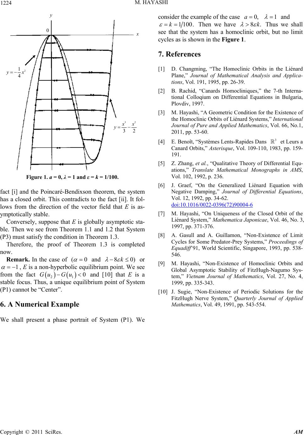 M. HAYASHI Copyright © 2011 SciRes. AM 1224 y 0 2 1 4 yx 32 32 x x y x Figure 1. a = 0, λ = 1 and ε = k = 1/100. fact [i] and the Poincaré-Bendixson theorem, the system has a closed orbit. This contradicts to the fact [ii]. It fol- lows from the direction of the vector field that E is as- ymptotically stable. Conversely, suppose that E is globally asymptotic sta- ble. Then we see from Theorem 1.1 and 1.2 that System (P3) must satisfy the condition in Theorem 1.3. Therefore, the proof of Theorem 1.3 is completed now. Remark. In the case of (0 and 80)k or 1 , E is a non-hyperbolic equilibrium point. We see from the fact 21 0Gu Gu and [10] that E is a stable focus. Thus, a unique equilibrium point of System (P1) cannot be “Center”. 6. A Numerical Example We shall present a phase portrait of System (P1). We consider the example of the case 0,a 1 and 1 100.k Then we have 8.k Thus we shall see that the system has a homoclinic orbit, but no limit cycles as is shown in the Figure 1. 7. References [1] D. Changming, “The Homoclinic Orbits in the Liénard Plane,” Journal of Mathematical Analysis and Applica- tions, Vol. 191, 1995, pp. 26-39. [2] B. Rachid, “Canards Homocliniques,” the 7-th Interna- tional Colloqium on Differential Equations in Bulgaria, Plovdiv, 1997. [3] M. Hayashi, “A Geometric Condition for the Existence of the Homoclinic Orbits of Liénard Systems,” International Journal of Pure and Applied Mathematics, Vol. 66, No.1, 2011, pp. 53-60. [4] E. Benoît, “Sy stè me s Lents-Rapides Dans 3 et Leurs a Canard Orbits,” Asterisque, Vol. 109-110, 1983, pp. 159- 191. [5] Z. Zhang, et al., “Qualitative Theory of Differential Equ- ations,” Translate Mathematical Monographs in AMS, Vol. 102, 1992, p. 236. [6] J. Graef, “On the Generalized Liénard Equation with Negative Damping,” Journal of Differential Equations, Vol. 12, 1992, pp. 34-62. doi:10.1016/0022-0396(72)90004-6 [7] M. Hayashi, “On Uniqueness of the Closed Orbit of the Liénard System,” Mathematica Japonicae, Vol. 46, No. 3, 1997, pp. 371-376. [8] A. Gasull and A. Guillamon, “Non-Existence of Limit Cycles for Some Predator-Prey Systems,” Proceedings of Equadiff’91, World Scientific, Singapore, 1993, pp. 538- 546. [9] M. Hayashi, “Non-Existence of Homoclinic Orbits and Global Asymptotic Stability of FitzHugh-Nagumo Sys- tem,” Vietnam Journal of Mathematics, Vol. 27, No. 4, 1999, pp. 335-343. [10] J. Sugie, “Non-Existence of Periodic Solutions for the FitzHugh Nerve System,” Quarterly Journal of Applied Mathematics, Vol. 49, 1991, pp. 543-554. |