 Applied Mathematics, 2011, 2, 1207-1212 doi:10.4236/am.2011.210168 Published Online October 2011 (http://www.SciRP.org/journal/am) Copyright © 2011 SciRes. AM A Parametric Linearization Approach for Solving Zero-One Nonlinear Programming Problems Asadollah Mahmoodzadeh Vaziri, A. V. Kamyad, S. Efatti Department of Ap pl i e d M athematics, Ferdowsi University of Mashhad, Mashhad, Iran E-mail: a_mvaziri@yahoo.com Received March 20, 2011; revised May 29, 2011; accepted June 6, 2011 Abstract In this paper a new approach for obtaining an approximation global optimum solution of zero-one nonlinear programming (0-1 NP) problem which we call it Parametric Linearization Approach (P.L.A) is proposed. By using this approach the problem is transformed to a sequence of linear programming problems. The ap- proximately solution of the original 0-1 NP problem is obtained based on the optimum values of the objec- tive functions of this sequence of linear programming problems defined by (P.L.A). Keywords: Zero-One Programming, Nonlinear Programming, Nonlinear Optimization 1. Introduction Integer programming is one of the most interesting and difficult research areas in mathematical programming and operations research. During the past years, many works has been devoted to linear integer programming, linear 0-1 programming and nonlinear 0-1programming problems [1-4]. Nnonlinear constrained integer programming problem have many applications in sciences and engineering. A number of research paper dealing with reliability opti- mization problems are reported in the literature. These are integer programming problems with nonlinear sepa- rable objective function and nonlinear multi choice con- strained [5,6]. A developed optimization method for solving integer nonlinear programming problem (INLP) with 0-1 vari- able could be found in [7]. This method is closely related to the lexicographic method of Gilmore and Gomory [8], for the knapsack problem and additive algorithm of Balas [9]. One of the conventional methods for solving zero-one nonlinear programming problem is to transform it to a linear programming problem. The main difficulty of this method is the very large number of variables and con- straints which increases the problem-size. A linearization involving a linear number of variables and constraints was first proposed by Glover [10] and improved by Oral and Kettani [11,12]. The resulting lin- earization involving only n – 1 additional variable and 2(n – 1) linear constraint. Hanssen and Meyer in [13] compare different ways for linearization the unconstraint quadratic zero-one mini- mization problem. This approaches involves to increase the number of variables and constraints. Consider the zero-one nonlinear programming prob- lem as follow: minimize subject to01,, 01, 0or11,, , s k j fx , xs hxk l m jn (1) where .: n f and ; .: n s g 1, , m and .: n; kk h1,, l a rete constraints re nonlinear functions. We can replace the discof the form 0 j x or 1; 1, ,jn , by the continuous new ones of 2 j xx the form0 j ; 1,,nj . It is trivial that this two constraintst we consider zero-one nonlinear programming problem in which the discrete constraint are replaced with continuous ones. Then we have the following nonlinear programming problem: s are equivalent. At fir 2 minimi ze subject to01,, 01, 01,, s k jj fx , , xs hxk l m xj n (2) In this paper we present a new approach call it para- metric linearization approach for finding the approxi-  A. M. VAZIRI ET AL. 1208 ond section contains a description of parametric lin . The Parametric Linearization Approach et mated global optimum of zero-one NP problem by solv- ing a sequence of linear programming problems over sub-regions. The solution of the sequence of LP prob- lems tends to the optimal solution of the original nonlin- ear problem. The reminder of the paper is organized as follow: The sec We call as a parametric piecewise linear ap- proximation o earization approximation and the convergence results. The third section contain a description of using the pa- rametric linearization approximation for solving zero-one nonlinear programming problem. In the forth section the approach will be followed to decrease the number of sub-problems which must be solved in each iteration. Numerical examples used to illustrate the efficiency of the proposed approach and they are given in fifth section. The last section draws overall conclusions. 2 L x that be a nonlinear smooth function on [a,b]. We knowthe linear Taylor expansion of x at the point 0[,] ab as follows: 000 x xfx , fx x where x0 be an arbitrary point in (a,b). In ual Taylor us expansion x0 is a fixed point but in our definition this is an arbitrary point. Thus we may call it moving linear Taylor expansion of x. Definition 2.1: Widere cons a partition of an interval [a,b] as the following form: ,Paba y , where ned by: 01 ,,, rr yy b 01 r yy y. orm of partition defiThe n ,maxPab y 01 1ririi y . Definition 2.2: Let x is a nonlinear function on [a,b] and , r ab bpartition of it. Let defined i e the x a plinear approximation of arametric x on terval sub-in 1 , ii y as follow: 1 ,&0,,1, iiii ii i xfsxfssfs xyy ir where 1 , iii yy we define is an arbitrary point. Now rx as the following G form: where 1 1 , 0ii r ri yy i Gxfx x , A ollowin is the characteristic function and defined as the fg: 1 0. A A x A (.) r G f x e on [a,b]. Note 2.following theorems it is shown that w 1: In th hen the norm of partition tends to zero it means ,0Pab r Gx is thenr uniformly convergent to x (the original nonlinear function). In the other word we may shown that: uniformly on, r Gf ab First we show that r Gf pointwise on [a,b]. Lemma 2.1: Let 01 1 ,,,,, rrr abay yyyb partition of [a, b]. If y is continuous is an arbitrary function on [a,b] and 1 ,, ii syy then : mi 0 li rii P sfsxs Definition 2.3: A family of complex fction f defined on the set A X is said to be eq fy . Proof: The proof is a simple conclusion of the defini- tion. in a metric space un uicontinuous on A if for every 0 there exist 0 such that fx fz whenever ,dxz , ,, zA .f Here ,dxz denote the metric of A (see [6]). Since r Gx is a sequence l that this seqntinuous. of linear function it is trivia ence is equico Theorem 2.1:Let u be an equicontinuous se- qutence of funcions on a compact set A and con- veint-wise rges poon A. Then converge uniformly on A. Proof: Since icontinuous on A then: is equ 00.., NN stdxzf xf z ,,1,2,.xz AN at forIt is trivial th each A and 0 we have , xA Nx . So , xA Nx mp Thus t oact set this ring. here is an open- exist the open-cov- A is a ccoverig ovepoint ering for A. Since have a finite sub-c 2 n 1 ,,, r in A such that 1 r i N , i A . There- fore for each A the1,2,,) iirre ( exist in A such that ,i dx and therefore: for1, 2,. NNi x f We know th fN at is pointwise ce se- quence theing a natural num convergen n there eber M such that for each we have: xist qMpM, 1 22 q qr pr ff 1p qp ff ff Therefore we have the following inequalities: Copyright © 2011 SciRes. AM  A. M. VAZIRI ET AL. Copyright © 2011 SciRes. AM 1209 3 qp qqiqi qqiqipipip fx fxfx ff ff fffx pipip f f fx fx Then according to the theorem 7.8 in [6] the sequence is uniformly continuous on A and the proof is leted. Theorem 2.2: Let comp r Gx is a piecewise linear ap- proximation of x on [a,b 1r ] as the following form: 1 , 0 . ii ri yy i Gx fxx Then: uniformly on, r Gf ab . Proof: The pmediate consequence of lemmroof is ima 2.1 and theorem 2.1. Let is nonlinear smooth function where a piecewise linear parametric ap- proximation for .:fA 1 n ii Aab roduce ,. n i Here we int x which is the exten of defini- tio nsio n 2.2. Definition 2.4: Consider the nonlinear smooth func- tion fA where 1, n ii i .: ab . Also con- A as follows: sider partition of ce A is M PA as a , 1 |, ,0,1, ,1, n Miin PA Aiir where 12 ,,i 121 2 , 1)1 , iiii n i A (3) Hen partitioned to M cells where 1 2 ,, ((1) ,, nn iiii . n r partition Let for shown the cell of this by 1, ,kM and 1 kk th k k E ,, n k ss w k is to shownt of usedn any poi k E. No x imation of is defi ned linear tric ap- as aparame prox x for k E as follows: | k k kxsk xfxxsfs where kk E for 1, , .kM ow G as a pricewise linear ap- ximation N is pro Mx of defined x on A as follows: M 1k Mk E k Gxfx x Note s note 2 2.2: A.1 we have 0 mM AGx fx . li M P 3. Description of the Approach Aach we consider the nonlinear programming problems whichre shown in (2). In our approach we introduce the parametric linearization approximation for nonlinear functions. For solving the optimization problem (2) the nonlinear objective func- tion and constraints are transformed approximately to the piecewise linear functions. We consider M PA of the cell [0 which is explained above be a artitions Without loss of generality region is rvals of tm ,1] . n p [0,1]n he for we can assume that this partition of the gular, it means that we have sub-intere 1 , j ii ; 1, ,jn and j ij ih where 1 hr and 0, j i t first for description our appro a 1, ,1r. We consider the nonlinear constraints of the form 20 jj xx , 1,, .jn By using the parametric lin- earization approach we may change approximately this constraint to the following form: 2 1x(1 ) (1) 20,, 1,, ,. 2 jj jj jj j ijijii ii i x jn After this according to the following manner in each sub-regionf the form ofay form the other linear functions in the optimization pr So each nonlinear functi o A,1]n we mtrans- 12 ,,, n ii i [0 non oblem (2) to the parametric linear approximation form. ons x; s x, 1,, m ; k hx, 1, ,kl in the 12 ,,ii A, n i sub-regions trans- formed approximately to the following parametric lin- ear form: 11 nn j jj jj xx ff fx f x ss nn 11 1, , ss j jj gg jj gx g x xx sm 11 kk nn kk j jj hh hx hx xx jj 1, ,kl where 12 ,,, n ii i such that (1) 2 jj j ii i , 1, ,jn and 1,, n xx such that (1) , j jii x . Therefore in each sub-region of the above form we have the following linear programming problem:  1210 A. M. VAZIRI ET AL. 1 11 11 2 (1) minimize subject to01,, 01,, 212 01,, ,1,, jj jj nn j j 1j jj ss nn js jj jj kk nn jk jj jj iji jii f xf x gg f x gsm xx hh hkl xx jn jn (4) For solving the above linear programming problem we divided the interval [0,1] to r equal sub-interval of the form 123 1 0,,,1 . r rrr r We know that in the solution of the optimization problem (3) all vari- ables must be equal zero or one. Therefore after dividing the interval [0, 1] we only should consider the first and the last sub-intervals 1 0, rr A and 1,1 rr r A . In these sub-intervals let 1 2 j ir and 21 2 j ir r so be shown in (4). Le ms be solved the optimum solut we have 2n linear programming problems of the form which t this linear programming proble ion and the opti- mal value of the objective function of this linear pro- gramming problems are shown with i and i z re- spectively then the optimal solution of the original opti- mization problem of the form (2) may be calculated as follows: min ni i zz 12 (5) ms and lemmas which are ٍAccording to the theore proved in Section 2, we know that if in any partitions of [0, 1] the norm of partitions tends to zero we have 0limRR A and lim 1 RR A Therefore if an arbitrary partition of [0, 1] be refined then each linear approximation of nonlinear functions x and s x; 1, , m and k hx; 1, ,kl tends to the values 0 , 0 s g; 1,, m; 0 k h; 1, ,kl and 1 and s g1; 1, , m and 1 k h; 1, ,kl and constraint of the form 20 j i ; 1, ,jn21 j ij x te According to the described approach nonlinear programming problems this problems must be converted to a sequence of linear programming problems. In this situation if n the number of variable in the main optimization problem is a large with 2n sub-problems which must be solved. According to the following manner this number may be decreased. At first the sub-problems are solved se- quentially until the first feasible solution has been deter- mined. For the reminder sub-regions by substituting xj with nds to values xj = 0 or xj = 1 which is the hole feasible solution of the original zero-one non-linear programming problem (2). 4. Decreasing the Number of Sub-Problems for solving zero-one number then we faced j i the objective function of the converted linear programming problem was calculated. If tulate ective fu thlinear problem is greatere obe functi e linear programming problem in ed with the older ones. This manner has w the effi- ci he calc value of the objnctions ofis program- ming than thjectivon of the feasible solution th this sub-region isn’t solved otherwise it be solved. After this if the solved problem has the feasible solu- tion the value of the objective function of this problem as substitutw been repeated until the sub-problems are ended. The aved value of the objective function and corresponding s design variable are the approximated answer for the main zero-one nonlinear programming problems. 5. Numerical Examples Now we give the numerical examples to sho ency of our proposed algorithm. Example 5.1: Consider the following zero-one nonlin- ear programming problem: 12 1 23 π n1sin sin1 x zex x 222 12 3 2 12 13 2 .. 2 21 3 st xxx xx xx 123 123 2 ,, 0,1 xxx xxx mi Copyright © 2011 SciRes. AM 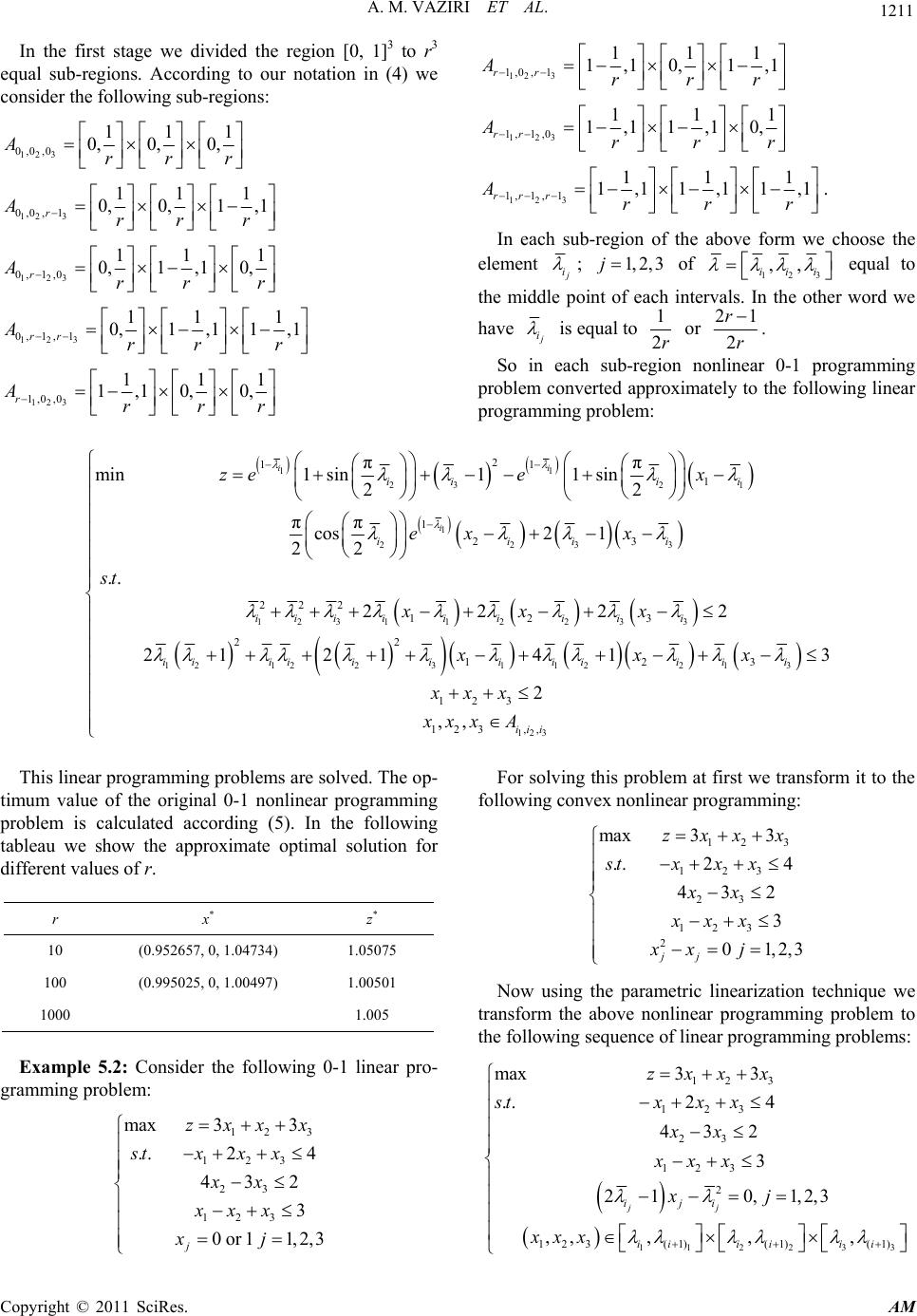 A. M. VAZIRI ET AL. 1211 In the first stage we divided the region [0, 1]3 to r3 equal sub-regions. According to our notation in (4) we consider the following sub-regions: 123 0,0 ,0 111 0, 0, 0,Arrr 12 3 0,0 ,1 11 0,0,1A 1 , 1 rrrr 123rrr 0, 1,0 11 1 0,1,10, r A 123 0, 1, 1 11 1 0 , 1,11,1 rr Arr r 123 1,0 ,0 11 1,10, 0, r Arr 12 3 1,0 ,1 111 1,10, 1,1 rr Arrr 123 1,1 ,0 11 1,11,10, rr Arr 1 r 123 1, 1, 1 111 1,11,11,1 rrr Arrr . In each sub-region of the above form we choose the element i ; 1, 2,3j of 123 ,, iii equal to the middle point of each intervals. In the other word we have i is equal to 1 2r or 21 2 r r . So in each sub-region nonlinear 0-1 programming problem converted approximately to the following linear programming problem: 1 r 11 232 1 1 2233 1 2 22 .. i st 2 3 112233 1212 2 2 11 1 1 23 22 12 3 22 ππ 1sin1 1sin 22 ππ cos2 1 22 2 2 21 21 min ii i iiii iiii ii iiiiii iiii i zee x ex x xxx 3112 213 123 123 12 3 123 ,, 41 3 2 ,, iiii iii iii xxx xxx xxx A This linear programming problemhe op- timum value of the original 0-1 nonlinear programming problem is calculated according (5). In the following tableau we show the approximate optimal solution for different values of r. r x* z* s are solved. T 10 (0.952657, 0, 1.04734) 1.05075 100 (0.995025, 0, 1.00497) 1.00501 1000 1.005 Example 5.2: Consider the following 0-1 linear pro- gramming problem: For solving this problem at first we transform it to the following convex nonlinear programming: 3 Now using the parametric linearization technique we transform the above nonlinear programming problem to the following sequence of linear programming problems: 123 123 23 123 max 33 ..2 4 432 3 0or1 1,2,3 j zxxx stxxx xx xxx xj 123 123 23 123 2 max 33 ..2 4 432 3 01,2, jj zxx x stxx x xx xxx xx j 112 23 3 123 123 23 123 2 123 (1)(1)(1) max33 ..2 4 432 3 210,1, 2,3 ,, ,,, jj iji ii iiii zxx x stxxx xx xxx xj xxx Copyright © 2011 SciRes. AM  1212 Here we consider r =10 and assuming that A. M. VAZIRI ET AL. 0.05 j i and 0.95 j i from the above sequence of linear pro- gramming problem we have 8 linear programming prob- lems for solving. After solving these problems on the sub-feasible region and constitute a set of the approxi- ate optimal solution of the sub-problems, the approxi- mate optimal solution of toriginal problem is obtained from followinlem: m he the g optimization prob 18 max ii z wher is the optimal vale of the objective function f the sub-problems. Then the approximate optimal solu- tio 028, 1.0028, 1.0028) with the opti- mal value of the objective function is and z* = 7.0194. 6. Conclusions In this paper we investigated the optimization technique for solving zero-one mixed nonlinear programming prob- lems. We obtained the global convergence for our ap- pr the zero-one nonlinear programming problems and then prop approach can be used for solved this problems. 7. References [1] P. Hansen, “Method of Nonlinear 0-1 Programming,” Annals of Discrete Mathematics, Vol. 5, 1979, pp. 53-70. [2] rial Optimization, Vol. 1, 1998, pp. 189-298. [3] G. L. Nemhauser and L. A. Wolsey, “Integer and Com binatorial Optimization,” John Wiley and Sons, New York, 1988. hes to Discrete Optimization Problems,” In: G. Di Pillo and F. Gianessi, Eds., Nonlinear Optimization and Applications, Plenum Publishing, New York, 1996, pp. 313-328. e i z o n of the original zero-one linear programming problem is obtained x* = (1.0 oach. Numerical examples are shown the effectiveness of the proposed algorithm. The nonlinear integer pro- gramming problems can be transformed to osed J. Mitchell, P. M. Pardalos and M. G. C. Resende, “Inte- rior Point Method for Combinatorial Optimization,” In: D. Z. Du and P. Paradalos, Eds., Handbook of Combinato- - [4] P. M. Paradalos, “Continuous Approac [5] M. S. Chern and R. H. Jan, “Reliability Optimization Problems with Multiple Constraints,” IEEE Transactions on Reliability, 1986, Vol. 35, No. 4, pp. 431-436. doi:10.1109/TR.1986.4335497 [6] K. B. Mira and U. Sharma, “An Efficient Algorithm to Solve Integer Programming Problems Arising in System- gn,” IEEE Transactions on Reliability, 991, pp. 81-91. Reliability Desi Vol. 40, No. 1, 1 [7] E. L. Lawlev and M. D. Bell, “A Method for Solving Discrete Optimization Problems,” Operations Research, Vol. 14, No. 6, 1966, pp. 1098-1112. doi:10.1287/opre.14.6.1098 [8] P. C. Gilmol and R. E. Gomory, “The Theory and Com- putation of Knapsack Function,” Operations Research, Vol. 14, 1966, pp. 1045-1074. doi:10.1287/opre.14.6.1045 [9] E. Balas, “An Additive Algorithm for Solving Linear Programs with 0-1 Variable,” Operations Research, Vol. , pp. 517-545. doi:10.1287/opre.13.4.51713, No. 4, 1965 0] F. Glover, “Improved Linear Integer Programming For-[1 mulations of Nonlinear Integer Problems,” Management Science, Vol. 22, No. 4, 1975, pp. 455-460. doi:10.1287/mnsc.22.4.455 [11] M. Oral and O. Kettani, “Reformulating Nonlinear Com- binatorial Optimization Problems for Higher Computa- tional Efficiency,” European Journal of Operational Re- search, Vol. 58, No. 2, 1992, pp. 236-249. doi:10.1016/0377-2217(92)90210-Z [12] M. Oral and O. Kettani, “A Linearization Procedure for act Lineariza- Quadratic and Cubic Mixed Integer Problems,” Opera- tions Research, Vol. 40, Supplement 1, 1992, pp. s109- s116. [13] P. Hansen and C. Meyer, “Improved Comp tions for the Unconstrained Quadratic 0-1 Minimization Problem,” Discrete Applied Mathematics, Vol. 157, 2009, pp. 1267-1290. doi:10.1016/j.dam.2007.12.008 Copyright © 2011 SciRes. AM
|