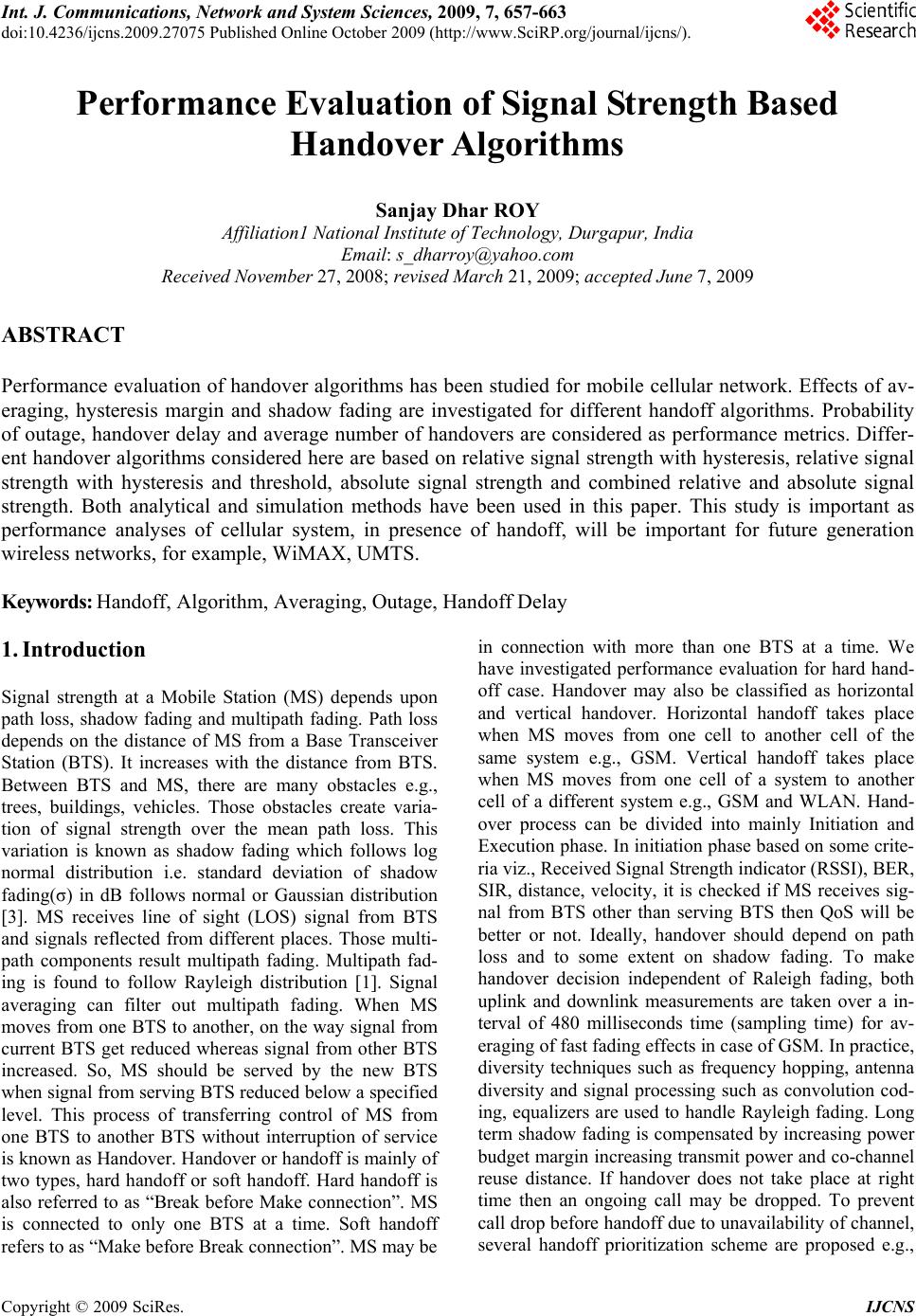Int. J. Communications, Network and System Sciences, 2009, 7, 657-663
doi:10.4236/ijcns.2009.27075 Published Online October 2009 (http://www.SciRP.org/journal/ijcns/).
Performance Evaluation of Signal Strength Based
Handover Algorithms
Sanjay Dhar ROY
Affiliation1 National Institute of Technology, Durgapur, India
Received November 27, 2008; revised March 21, 2009; accepted June 7, 2009
ABSTRACT
Performance evaluation of handover algorithms has been studied for mobile cellular network. Effects of av-
eraging, hysteresis margin and shadow fading are investigated for different handoff algorithms. Probability
of outage, handover delay and average number of handovers are considered as performance metrics. Differ-
ent handover algorithms considered here are based on relative signal strength with hysteresis, relative signal
strength with hysteresis and threshold, absolute signal strength and combined relative and absolute signal
strength. Both analytical and simulation methods have been used in this paper. This study is important as
performance analyses of cellular system, in presence of handoff, will be important for future generation
wireless networks, for example, WiMAX, UMTS.
Keywords: Handoff, Algorithm, Averaging, Outage, Handoff Delay
1. Introduction
Signal strength at a Mobile Station (MS) depends upon
path loss, shadow fading and multipath fading. Path loss
depends on the distance of MS from a Base Transceiver
Station (BTS). It increases with the distance from BTS.
Between BTS and MS, there are many obstacles e.g.,
trees, buildings, vehicles. Those obstacles create varia-
tion of signal strength over the mean path loss. This
variation is known as shadow fading which follows log
normal distribution i.e. standard deviation of shadow
fading(σ) in dB follows normal or Gaussian distribution
[3]. MS receives line of sight (LOS) signal from BTS
and signals reflected from different places. Those multi-
path components result multipath fading. Multipath fad-
ing is found to follow Rayleigh distribution [1]. Signal
averaging can filter out multipath fading. When MS
moves from one BTS to another, on the way signal from
current BTS get reduced whereas signal from other BTS
increased. So, MS should be served by the new BTS
when signal from serving BTS reduced below a specified
level. This process of transferring control of MS from
one BTS to another BTS without interruption of service
is known as Handover. Handover or handoff is mainly of
two types, hard handoff or soft handoff. Hard handoff is
also referred to as “Break before Make connection”. MS
is connected to only one BTS at a time. Soft handoff
refers to as “Make before Break connection”. MS may be
in connection with more than one BTS at a time. We
have investigated performance evaluation for hard hand-
off case. Handover may also be classified as horizontal
and vertical handover. Horizontal handoff takes place
when MS moves from one cell to another cell of the
same system e.g., GSM. Vertical handoff takes place
when MS moves from one cell of a system to another
cell of a different system e.g., GSM and WLAN. Hand-
over process can be divided into mainly Initiation and
Execution phase. In initiation phase based on some crite-
ria viz., Received Signal Strength indicator (RSSI), BER,
SIR, distance, velocity, it is checked if MS receives sig-
nal from BTS other than serving BTS then QoS will be
better or not. Ideally, handover should depend on path
loss and to some extent on shadow fading. To make
handover decision independent of Raleigh fading, both
uplink and downlink measurements are taken over a in-
terval of 480 milliseconds time (sampling time) for av-
eraging of fast fading effects in case of GSM. In practice,
diversity techniques such as frequency hopping, antenna
diversity and signal processing such as convolution cod-
ing, equalizers are used to handle Rayleigh fading. Long
term shadow fading is compensated by increasing power
budget margin increasing transmit power and co-channel
reuse distance. If handover does not take place at right
time then an ongoing call may be dropped. To prevent
call drop before handoff due to unavailability of channel,
several handoff prioritization scheme are proposed e.g.,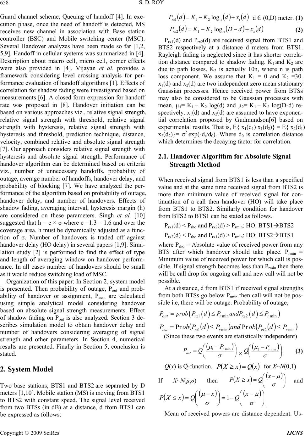

S. D. ROY 658
Guard channel scheme, Queuing of handoff [4]. In exe-
cution phase, once the need of handoff is detected, MS
receives new channel in association with Base station
controller (BSC) and Mobile switching center (MSC).
Several Handover analyzes have been made so far [1,2,
5,9]. Handoff in cellular systems was summarized in [4].
Description about macro cell, micro cell, corner effects
were also provided in [4]. Vijayan et al. provides a
framework considering level crossing analysis for per-
formance evaluation of handoff algorithms [1]. Effects of
correlation for shadow fading were investigated based on
measurements [6]. A closed form expression for handoff
rate was proposed in [8]. Handover initiation can be
based on various approaches viz., relative signal strength,
relative signal strength with threshold, relative signal
strength with hysteresis, relative signal strength with
hysteresis and threshold, prediction technique, distance,
velocity, combined relative and absolute signal strength
[7]. Our approach considers relative signal strength with
hysteresis and absolute signal strength. Performance of
handover algorithm can be determined based on criteria
viz., number of unnecessary handoffs, probability of
outage, average number of handoffs, handover delay, and
probability of blocking [7]. We have analyzed the per-
formance of the algorithm based on probability of outage,
handover delay, and number of handovers. Effects of
shadow fading, averaging interval, hysteresis margin (h)
are considered on these parameters. Singh et al. [10]
suggested that h = e × σ where e =1.3 – 1.6 and over the
coverage area, h must be dynamically adjusted as a func-
tion of σ. Number of handovers is traded off against
handover delay (HO delay) in several papers [1,9]. Simu-
lation study [2] is performed to find the effect of type
and length of averaging window on handover perform-
ance. In all cases number of handovers should be small
as it would reduce switching load of MSC.
Organization of this paper: In Section 2, system model
is presented. Then probability of outage, Pout and prob-
ability of handover or assignment, Passn are calculated
using simple analytical model considering handover
based on absolute signal strength measurements. Effect
of shadow fading on Pout is also analyzed. Section 3 de-
scribes simulation model to obtain handover delay and
number of handovers considering averaging of signal
strength and other parameters. In Section 4, numerical
results are presented. Finally in Section 5, conclusion is
stated.
2. System Model
Two base stations, BTS1 and BTS2 are separated by D
meters [1,10]. Mobile station (MS) is moving from BTS1
to BTS2 with constant speed. The signal level received
from two BTSs (in dB) at a distance, d from BTS1 can
be expressed as follows:



 dxdKKdP
rx 110
log
211 



d Є (0,D) meter. (1)



 dxdDKKdP
rx 210
log
212 



(2)
Prx1(d) and Prx2(d) are received signal from BTS1 and
BTS2 respectively at a distance d meters from BTS1.
Rayleigh fading is neglected since it has shorter correla-
tion distance compared to shadow fading. K1 and K2 are
due to path losses. K2 is actually 10n, where n is path
loss component. We assume that K1 = 0 and K2 =30.
x1(d) and x2(d) are two independent zero mean stationary
Gaussian processes. Hence received power from BTSs
may also be considered to be Gaussian processes with
mean, µ1= K1 – K2 log(d) and µ2= K1 – K2 log(D-d) re-
spectively. x1(d) and x2(d) are assumed to have exponen-
tial correlation proposed by Gudmundson[6] based on
experimental results. That is, E{ x1(d1) x1(d2)} = E{ x2(d1)
x2(d2)}= σ2
exp(-ds/d0). Where d0 is correlation distance
which determines the decaying factor for correlation.
2.1. Handover Algorithm for Absolute Signal
Strength Method
When received signal from BTS1 is less than a specified
value and at the same time received signal from BTS2 is
more than minimum value of received signal for con-
tinuation of a call then handover (HO) will take place
from BTS1 to BTS2. Similarly condition for handover
from BTS2 to BTS1 can be stated as follows.
Prx1(d) < Prho and Prx2(d) > Prmin: HO: BTS1BTS2
Prx2(d) < Prho and Prx1(d) > Prmin: HO: BTS2BTS1
where Prho = Absolute value of received power from any
BTS after which handover should take place. Prmin =
Minimum value of received power for which call is pos-
sible. If signal strength becomes less than Prmin then there
will be call drop for ongoing call and new call will not be
possible.
At a distance, d from BTS1 if received signal strengths
from both BTSs go below Prmin then call will not be pos-
sible i.e, there will be outage. Probability of outage,




1min 2minoutrxr rxr
P probPdPandPdP 




min2min1 PrPr rrxrrxout PdPobandPdPobP



(Since these two events are statistically independent)











min1 r
out
P
QP 










min2 r
P
Q
(3)
Q(x) is Q-function.

 xQxXP   for X~N(0,1)
If X~N(μ,σ) then











 x
QxXPand




















 x
Q
x
QxXP 1
.
Mean of received powers are distance dependent. Us-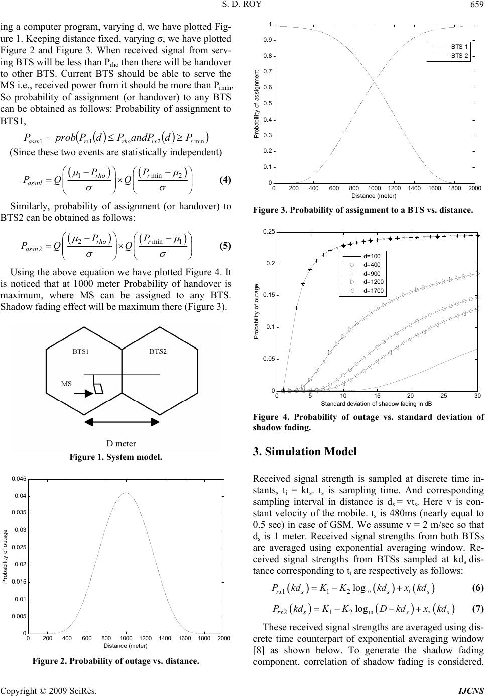

S. D. ROY 659
ing a computer program, varying d, we have plotted Fig-
ure 1. Keeping distance fixed, varying σ, we have plotted
Figure 2 and Figure 3. When received signal from serv-
ing BTS will be less than Prho then there will be handover
to other BTS. Current BTS should be able to serve the
MS i.e., received power from it should be more than Prmin.
So probability of assignment (or handover) to any BTS
can be obtained as follows: Probability of assignment to
BTS1,
 
min211 rrxrhorxassn PdandPPdPprobP 
(Since these two events are statistically independent)
 
1min 2 rho r
assnl
PP
PQ Q


 

 


 (4)
Similarly, probability of assignment (or handover) to
BTS2 can be obtained as follows:


2min 1
2
rho r
assn
PP
PQ Q


 

 

 

(5)
Using the above equation we have plotted Figure 4. It
is noticed that at 1000 meter Probability of handover is
maximum, where MS can be assigned to any BTS.
Shadow fading effect will be maximum there (Figure 3).
Figure 1. System model.
0200 400600 8001000 1200 14001600 1800 2000
0
0.005
0.01
0.015
0.02
0.025
0.03
0.035
0.04
0.045
Dis t ance (met er)
P robabili t y of outage
Figure 2. Probability of outage vs. distance.
02004006008001000 1200 14001600 18002000
0
0.1
0.2
0.3
0.4
0.5
0.6
0.7
0.8
0.9
1
Dis tance (met er)
Probabilit y of ass ignment
BTS 1
BTS 2
Figure 3. Probability of assignment to a BTS vs. distance.
05 10 15 20 2530
0
0. 0 5
0.1
0. 1 5
0.2
0. 2 5
Standard deviat ion of s hadow fading in dB
Probabi l i ty of outage
d= 100
d= 400
d= 900
d= 1200
d= 1700
Figure 4. Probability of outage vs. standard deviation of
shadow fading.
3. Simulation Model
Received signal strength is sampled at discrete time in-
stants, ti = kts. ts is sampling time. And corresponding
sampling interval in distance is ds = vts. Here v is con-
stant velocity of the mobile. ts is 480ms (nearly equal to
0.5 sec) in case of GSM. We assume v = 2 m/sec so that
ds is 1 meter. Received signal strengths from both BTSs
are averaged using exponential averaging window. Re-
ceived signal strengths from BTSs sampled at kds dis-
tance corresponding to ti are respectively as follows:


10 1 112
log
rx sss
PkdKKkd xkd 

(6)


10 2 212
log
rx sss
PkdKKDkdxkd

(7)
These received signal strengths are averaged using dis-
crete time counterpart of exponential averaging window
[8] as shown below. To generate the shadow fading
component, correlation of shadow fading is considered.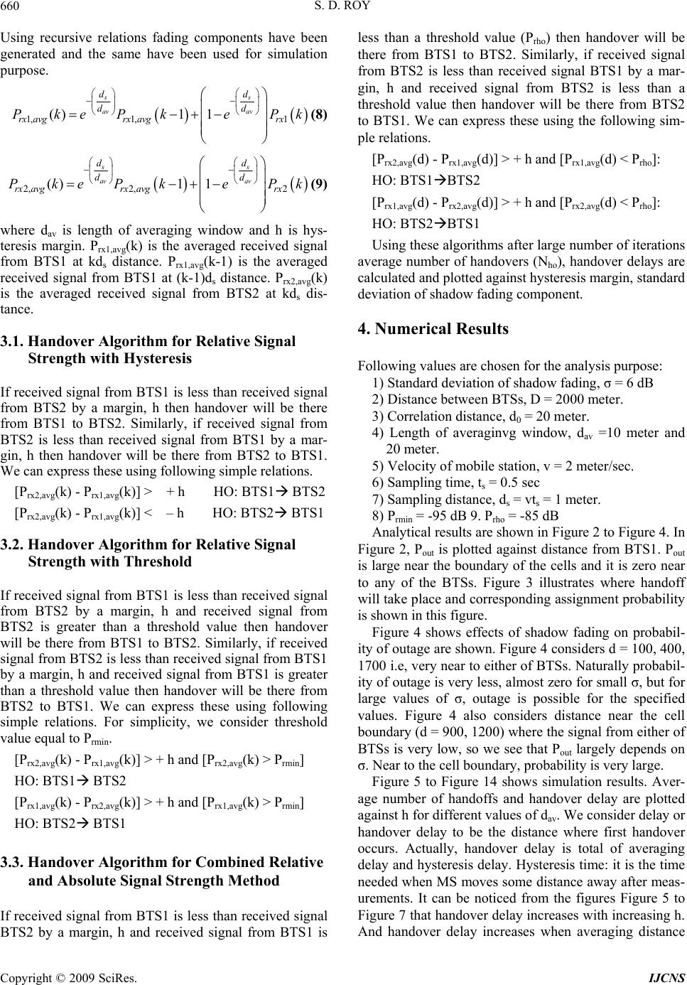

S. D. ROY 660
Using recursive relations fading components have been
generated and the same have been used for simulation
purpose.
 
1, 1,1
()1 1
s
av av
d
dd
rx avgrx avgrx
PkeP keP
 

 
 






s
d
k (8)
 
2, 2,2
()1 1
s
av av
dd
dd
rx avgrxavgrx
PkeP keP
 

 
 






s
k (9)
where dav is length of averaging window and h is hys-
teresis margin. Prx1,avg(k) is the averaged received signal
from BTS1 at kd
s distance. Prx1,avg(k-1) is the averaged
received signal from BTS1 at (k-1)ds distance. Prx2,avg(k)
is the averaged received signal from BTS2 at kds dis-
tance.
3.1. Handover Algorithm for Relative Signal
Strength with Hysteresis
If received signal from BTS1 is less than received signal
from BTS2 by a margin, h then handover will be there
from BTS1 to BTS2. Similarly, if received signal from
BTS2 is less than received signal from BTS1 by a mar-
gin, h then handover will be there from BTS2 to BTS1.
We can express these using following simple relations.
[Prx2,avg(k) - Prx1,avg(k)] > + h HO: BTS1 BTS2
[Prx2,avg(k) - Prx1,avg(k)] < – h HO: BTS2 BTS1
3.2. Handover Algorithm for Relative Signal
Strength with Threshold
If received signal from BTS1 is less than received signal
from BTS2 by a margin, h and received signal from
BTS2 is greater than a threshold value then handover
will be there from BTS1 to BTS2. Similarly, if received
signal from BTS2 is less than received signal from BTS1
by a margin, h and received signal from BTS1 is greater
than a threshold value then handover will be there from
BTS2 to BTS1. We can express these using following
simple relations. For simplicity, we consider threshold
value equal to Prmin.
[Prx2,avg(k) - Prx1,avg(k)] > + h and [Prx2,avg(k) > Prmin]
HO: BTS1 BTS2
[Prx1,avg(k) - Prx2,avg(k)] > + h and [Prx1,avg(k) > Prmin]
HO: BTS2 BTS1
3.3. Handover Algorithm for Combined Relative
and Absolute Signal Strength Method
If received signal from BTS1 is less than received signal
BTS2 by a margin, h and received signal from BTS1 is
less than a threshold value (Prho) then handover will be
there from BTS1 to BTS2. Similarly, if received signal
from BTS2 is less than received signal BTS1 by a mar-
gin, h and received signal from BTS2 is less than a
threshold value then handover will be there from BTS2
to BTS1. We can express these using the following sim-
ple relations.
[Prx2,avg(d) - Prx1,avg(d)] > + h and [Prx1,avg(d) < Prho]:
HO: BTS1BTS2
[Prx1,avg(d) - Prx2,avg(d)] > + h and [Prx2,avg(d) < Prho]:
HO: BTS2BTS1
Using these algorithms after large number of iterations
average number of handovers (Nho), handover delays are
calculated and plotted against hysteresis margin, standard
deviation of shadow fading component.
4. Numerical Results
Following values are chosen for the analysis purpose:
1) Standard deviation of shadow fading, σ = 6 dB
2) Distance between BTSs, D = 2000 meter.
3) Correlation distance, d0 = 20 meter.
4) Length of averaginvg window, dav =10 meter and
20 meter.
5) Velocity of mobile station, v = 2 meter/sec.
6) Sampling time, ts = 0.5 sec
7) Sampling distance, ds = vts = 1 meter.
8) Prmin = -95 dB 9. Prho = -85 dB
Analytical results are shown in Figure 2 to Figure 4. In
Figure 2, Pout is plotted against distance from BTS1. Pout
is large near the boundary of the cells and it is zero near
to any of the BTSs. Figure 3 illustrates where handoff
will take place and corresponding assignment probability
is shown in this figure.
Figure 4 shows effects of shadow fading on probabil-
ity of outage are shown. Figure 4 considers d = 100, 400,
1700 i.e, very near to either of BTSs. Naturally probabil-
ity of outage is very less, almost zero for small σ, but for
large values of σ, outage is possible for the specified
values. Figure 4 also considers distance near the cell
boundary (d = 900, 1200) where the signal from either of
BTSs is very low, so we see that Pout largely depends on
σ. Near to the cell boundary, probability is very large.
Figure 5 to Figure 14 shows simulation results. Aver-
age number of handoffs and handover delay are plotted
against h for different values of dav. We consider delay or
handover delay to be the distance where first handover
occurs. Actually, handover delay is total of averaging
delay and hysteresis delay. Hysteresis time: it is the time
needed when MS moves some distance away after meas-
urements. It can be noticed from the figures Figure 5 to
Figure 7 that handover delay increases with increasing h.
And handover delay increases when averaging distance

S. D. ROY 661
0246810 1
2
600
700
800
900
1000
1100
1200
1300
Hyst eres i s (dB)
Average Crossover Poi nt (m et er)
dav = 10
dav = 30
Figure 5. Handover delay vs. hysteresis margin for relative
signal strength with hysteresis.
0 2 46 810 12
600
700
800
900
1000
1100
1200
1300
1400
Hyst eres i s (dB)
Average Crossover Poi nt (m et er)
T = -85 & dav = 10
T = -85 & dav = 30
T = -95 & dav = 10
T = -95 & dav = 30
Figure 6. Handover delay vs. hysteresis margin for relative
signal strength with threshold and hysteresis.
is increased. Since more averaging consumes more time.
There is no significant change in handover delay (with
dav =30) with respect to σ after considering its correlation.
That is due to averaging of signal strength. Averaging of
signals filter out multipath component and to some ex-
tent shadow fading variation. For this reason delay vs. σ
plot is not shown. Figure 5 shows variation of handoff
delay for relative RSS for dav =10 and 30. Handoff oc-
curs near to cell boundary for dav = 10 and h = 12. Hys-
tersis value is to be very large for avoiding ping-pong for
this algorithm. Figure 6 shows variation of crossover
point for relative signal strength with hystersis and
threshold. Four curves have been plotted for different
threshold and dav values. Handover delay will not change
with T for large values of h and dav. For example, at h
=12 and dav =30, handoff delays for T = -85 and -95 are
same.
Figure 7 shows handover delay for combined relative
and absolute signal strength based algorithm (CSS).
Handover delay is more for T = -95 dB as this allows MS
to be connected to the serving BTS for long compared to
that with T = -85 dB. Crossover point is more with dav =
30 than with dav = 10 meter because of large averaging.
It is observed that numbers of handoffs are less for
large values of hysteresis. For dav =30, number of hand-
offs is almost equal to one i.e, no unnecessary handovers
for the specified values. For dav =10, number of handoffs
is large. That means less averaging may lead to unneces-
sary handoffs. Figure 8 shows number of handoff vs.
hysteresis for relative signal strength basesd algorithm.
Number of handoff is less for dav = 30 meter due to large
averaging window length. Figure 9 shows variation of
Nho with h for CSS algorithm for different values of T
and dav. Number of handoff is lowest for T = -95 dB and
dav = 30. This happens because the current BTS keeps
control of MS for longer time. Figure 10 shows variation
0246810 12
600
700
800
900
1000
1100
1200
1300
1400
Hyst eres i s (dB)
Average Crossover Poi nt (m et er)
T = -95 & dav = 10
T = -95 & dav = 30
T = -85 & dav = 10
T = -85 & dav = 30
Figure 7. Handover delay vs. hysteresis margin for com-
bined relative & absolute signal strength with hysteresis
method.
0246810 12 14 1618
0
2
4
6
8
10
12
14
Hy st eresis (dB)
Average number of hando ffs
dav=10
dav=30
Figure 8. Average number of handoff vs. hysteresis margin
for relative RSS.

S. D. ROY 662
of Nho with h for relative signal strength with threshold
and hysteresis based algorithm for different values of T
and dav. Number of handoff is lowest for T = -85 dB and
dav = 30. This happens because the current BTS keeps
control of MS for longer time and control is transferred
to candidate BTS only after it provides very good signal
strength to sustain good quality and avoid ping pong. We
have analyzed three different handover algorithms. Re-
sults suggest that effect of σ, h and dav similar for all dif-
ferent algorithms.
Next three figures show tradeoff curves for all three
different handoff algorithms considered in this paper. Fig
11 show tradeoff for relative signal strength based hand-
off algorithm. Tradeoff curve provides an idea for
choosing handover design parameter. Handoff parameter
may be chosen for point where Nho and Cross over point
both are low. Figure 12 shows tradeoff for CSS algorithm
0 2 4 6 81012 14 1618 20
0
2
4
6
8
10
12
14
Hysteres i s (dB )
A verage number of handof fs
dav=10 & T = -85
dav=30 & T = -85
dav=10 & T = -95
dav=30 & T = -95
Figure 9. Average number of handoff vs. hysteresis margin
for CSS.
0 2 4 6 810 12 14
0
2
4
6
8
10
12
14
Hyst eres i s (dB)
A v erage number of handof fs
dav=10 & T = -95
dav=30 & T = -95
dav=10 & T = -85
dav=30 & T = -85
Figure 10. Average number of handoff vs. hysteresis margin
for relative signal strength with threshold and hysteresis.
0 2 4 6 810 12 14
600
700
800
900
1000
1100
1200
1300
Number of handoff
Average Cros sov er Point (m eter)
Relat i ve dav = 10
Relat i ve dav = 30
Figure 11. Tradeoff for relative RSS based algorithm.
0246810 12 14
600
700
800
900
1000
1100
1200
1300
1400
Number of handoff
Average Cros sover Point (m eter)
CSS T = -95 & dav = 10
CSS T = -95 & dav = 30
CSS T = -85 & dav = 10
CSS T = -85 & dav = 30
Figure 12. Tradeoff for relative CSS based algorithm.
for different values of dav and T. Nho is one when cross
over point is almost 1100 meter. Hence CSS algorithm
provides very good balance between two conflicting pa-
rameters Nho and handoff delay. Figure 12 shows trade-
off for relative signal strength with threshold and hys-
teresis based algorithm for different values of dav and T.
Nho is one when cross over point is almost 1200 meter.
Finally, Figure 14 shows tradeoff curve for all three dif-
ferent algorithms. Two algorithms other than relative
signal strength based handoff algorithm, provides almost
same performance with proper choice of hysteresis value.
Crossover point can be around 1200 meters with proper
setting of hystersis value for Nho = 1 (one).
5. Conclusions
This paper presents very simple method to choose hand-
over design parameters (e.g., averaging window length,
hysteresis margin, standard deviation of shadow fading)
for Mobile Cellular system. It uses analytical method for
finding probability of outage and it uses simulation

S. D. ROY 663
method for finding handover delay and average number
of handoffs. Analysis and simulation results are obtained
for three different algorithms. Absolute signal strength
based algorithm has to be considered for intersystem
handoff, as relative measurements are not possible for
different cellular systems because of their different
power requirement and other criteria. If candidate signal
strength is not large enough then there may be ping-pong
effect. Relative signal strength with hysteresis and
threshold takes care of this. If serving BS strength is
enough to provide good quality of service then a handoff
to candidate BS may be considered as unnecessary.
Hence, a combined absolute and relative signal strength
based handoff algorithm can take care of this problem.
Both of these two algorithms prevent unnecessary hand-
off by increasing handoff delay to some extent. Handoff
decision criteria can be critical when cell splitted (mi-
crocellular) to increase capacity and decrease power re-
quirements of MS. When there is very small hysteresis
margin or no hysteresis there may be ping-pong effect.
Due to dynamic behaviour of propagation environment
MS very close to BTS may be in deep fade for very short
duration (e.g., street corner effect). Handover should not
occur in such cases. To avoid this, averaging of signal
strength may be done over short duration while keeping
large hysteresis margin. Overlay macro cell may also be
employed to overcome this problem. For microcellular
systems short averaging time and large hystersis margin
is more reliable and reverse for macro cellular systems.
Probability of outage increases with increase in shadow
fading. Since designer has almost no control over the
shadow fading component, hysteresis margin can be dy-
namically varied to compensate the effect of shadow
fading.
6. Acknowledgments
The author would like to thank Mr. A. Chandra, Dr. S.
Kundu and Dr. S. K. Datta of NIT, Durgapur, India for
their valuable suggestions.
0 2 4 6 81012 14
600
700
800
900
1000
1100
1200
1300
1400
Number of handoff
Average Crossov er Poi nt (m eter)
Relat i ve THd T = -85 & dav = 10
Relat i ve Thd dav = 30
Relat i ve THd T = -95 & dav = 10
Relat i ve Thd T = -95 & dav = 30
7. References
[1] R. Vijayan and J. Holtzman, “A model for analyzing
handoff algorithms,” IEEE Transactions on Vehicular
Technology, Vol. 42, No. 3, pp. 351–356, August 1993.
[2] G. E. Corazza, et al., “Characterization of handover ini-
tialization in cellular mobile radio networks,” IEEE VTC’
94, pp. 1869–1872, 1994.
[3] T. S. Rappaport, “Wireless communications,” Prentice
Hall, 1996.
[4] D. Nisith, et al., “Handoff in cellular systems,” IEEE
Personal Communications, Dec. 1998.
[5] M. Gudmundson, “Analysis of Handover algorithm”,
IEEE VTC, May 1991, pp 537–42
Figure 13. Tradeoff for relative RSS with threshold based
algorithm. [6] M. Gudmundson, “Correlation model for shadow fading
in mobile radio systems,” Electronics Letters, Vol. 27, No.
23, pp. 2145–2146, November 1991.
0246810 12 14
600
700
800
900
1000
1100
1200
1300
1400
Number of handoff
Average Crossov er P oi nt (meter)
Relat i ve dav = 10
Relat i ve dav = 30
Relat i ve THd T = -85 & dav = 10
Relat i ve Thd dav = 30
CSS T = -95 & dav = 10
CS S d av = 3 0
[7] G. P. Pollini, “Trends in handover design,” IEEE Com-
munication Magazine, Vol. 34, pp. 82–90, March 1996.
[8] G. P. Pollini, “Handover rate in cellular systems: To-
wards a closed form approximation,” Global Telecom-
munications Conference, GLOBE COM’97, IEEE, Vol. 1,
pp. 711–715, November 1997.
[9] N. Zhang and J. M. Holtzman, “Analysis of handover
algorithms using both absolute and relative measure-
ments,” IEEE VTC’94, pp. 82–86, 1994.
[10] B. Singh, et al., “Sensitivity analysis of handover per-
formance to shadow fading in microcellular systems,”
IEEE ICPWC, 2005.
[11] S. D. Roy, “Effects of averaging, shadow fading and
hysteresis margin on handover performance,” CD pro-
ceedings, ICEMC, Pesit, Bangalore, Aug. 2007.
Figure 14. Tradeoff for all three algorithms together.