American Journal of Oper ations Research, 2011, 1, 134-146
doi:10.4236/ajor.2011.13015 Published Online September 2011 (http://www.SciRP.org/journal/ajor)
A Hierarchical Methodology for Performance Evaluation
Based on Data Envelopment Analysis: The Case of
Companies’ Competitiveness in an Economy
Mohamed Dia1, Fouad Ben Abdelaziz2
1School of Commerce and Administration, Laurentian University, Sudbury, Canada
2ESM Graduate Program, American University of Sharjah, Sharjah, UAE
Received July 22, 201 1; revised August 17, 2011; accepted September 7, 201 1
Abstract
In this research, we present a hierarchical Data Envelopment Analysis (DEA) methodology for competitive-
ness analysis. This methodology takes into account the heterogeneity of the decision making units (DMUs)
as well as the diversity of the comparison criteria. We propose to homogenize the DMUs by grouping them
hierarchically, which permits a better identification and definition of the criteria in each specific grouping.
The methodology proceeds first by the determination of the performances or relative efficiencies, which are
in turn aggregated into competitiveness indices in each grouping by the superiority index of [1]; then, the
overall competitiveness indices are determined additively along the hierarchical levels. We illustrate the
methodology by a competitiveness analysis of several companies belonging to different sectors of activity in
an economy, where are suggested ways of improvement for the non-competitive companies within their sec-
tors and within the economy.
Keywords: Data Envelopment Analysis, Heterogeneity, Hierarchies, Competitiveness Analysis
1. Introduction
As there is no perfect system to effectively evaluate the
competitiveness of a company, managers typically use a
range of measures of a financial and non-financial nature,
both internal and external. The importance and popular-
ity of these measures vary considerably over time and
from one company to another. The typical approach con-
sists, in most cases, in identifying the same measures of
competitiveness for each company, measuring them in
the same manner, and calculating an index of competi-
tiveness for each firm using a given model. This ap-
proach is acceptable if these companies are fairly homo-
geneous but it becomes inappropriate if the ho mogeneity
of the companies is not evident. This is the case if the
companies belong to different sectors or to different en-
vironments (countries, regions, economic areas, etc.).
Indeed, in today's world, it would be illogical to evaluate
biotech, electronic, aeronautical, agricultural, or textile
companies using the same indicators of competitiveness
and in the same way.
Data Envelopment An alys is [2 ] is a tech niqu e fo r meas-
uring performance, which is defined in this research as a
relative efficiency. Its application in competitiveness
analysis was suggested for the first time by [3]. Subse-
quently, [4] proposed using the model of [5] to measure
the competitiveness of nations, and [6] used the Moving
Frontier Analysis to perform a competitiveness analysis
of high-tech factories. All these studies have demon-
strated that DEA was appropriate for the study of com-
petitiveness analysis problems because it provides,
through the principle of data envelopment, a reference
for current and potential comparison to organizations for
effective formulations of competitiveness strategies.
However, evaluating the competitiveness of compa-
nies requires the selection of the most appropriate com-
petitiveness indicators and the use of ap propriate models.
These determinants are usually multiple and very diverse
and, as the company is not an isolated actor in its envi-
ronment, its competitiveness is influenced by the indus-
try and the nation. Indeed, [7] state that sector member-
ship of a company is a source of influence on the poten-
tial competitiveness of this company. For its part, [8,9]
argues that the environment in which firms operate af-

M. DIA ET AL.
135
fects significantly their competitiveness and that of their
industries. Meanwhile, [10] suggests that it is useful to
consider competitiveness at three different levels of ag-
gregation: the enterprise, the indu stry, and the country as
a whole. For each level of aggregation corresponds vari-
ous indicators of competitiveness that differs depending
on whether it is economic growth or the current and fu-
ture well-being of a company, a sector or a country that
is under consideration. It is to be noted also that some
notions of co mpetitiveness only apply to a given level of
aggregation and not to others.
Our study is considered within this context and pro-
poses an approach to measure the competitiveness of
heterogeneous companies in an economy where, it is
important to take into consideration both their basic and
specific characteristics of companies under consideration.
We propose, therefore, following the approaches advo-
cated by [7-10] to use a tree structure with three levels
(company, industry and economy) to better identify the
competitiveness indicators of companies in an economy.
The competitiveness of a comp an y in an econ o my is then
a combination of the competitiveness of its sector within
this economy and the competitiveness of the specific
company in this sector. Two key points underlie this ap-
proach. First, a company’s industry membership has a
decisive influence on its competitiveness, not only within
its own economy, but also by comparison with the same
sector in different economies [7,8,10,11]. Second, some
companies’ competitiveness indicators are valid only for
certain sectors and the same for those of sectors in cer-
tain economies [8-10]. In addition, the common indica-
tors may not necessarily have the same importance for
one company in comparison to another, especially if
these companies come from different sectors within dif-
ferent economies. Indeed, in such situations, the tech-
nologies used on both sides are different and character-
ized by the industry or the economy. Our methodology is
the first one, to our knowledge, to propose an analytical
model to measure the competiveness of heterogeneous
companies, and also the first one using a hierarchical
structure in DEA in this context.
Our proposed model, which is based on the DEA tech-
nique [2], meets the need expressed by [12] for a formal
model-based approach to competitiveness analysis that
managers or policy makers can use for strategic decision
making. However, given that DEA is designed to evalu-
ate homogeneous units, we propose to adapt the tech-
nique into a tree representation form with two grouping
levels (economy and sectors) so as to homogenize the
data in each level. Our approach is also the first one to
propose an explicit way to homogenize the DMUs in
DEA by adopting a hierarchical structure when there are
heterogeneity problems. The conceptual hierarchical struc-
ture of our problem is presented in Figure 1 where the
economy consists of n sectors evaluated on c perform-
ance criteria and where for each sector s, there are ns
companies evaluated on cs performance criteria. To our
knowledge, no study has so far treated a similar concep-
tual and methodological structu re, although some studies
using DEA in hierarchically structured problems have
been conducted [13-16]. For example, [14,16] evaluated
the relative efficiency of several power stations, each
consisting of several units and defined same inputs-out-
puts for the units and the power stations with few specif-
ics for the latter. The inputs-outputs shared between
power stations and power units were aggregated addi-
tively to the top level of the hierarchy to assess the rela-
tive efficiency of the power stations. In turn, [15] used an
approach similar to that of [14] and [16] where the units
and sub-units were, respectively, the universities and
their faculties or departments. For their part, [13] pro-
vided a classification of the DEA models that had as-
sessed DMUs whose internal structure was know and
could be represented as hierarchical networks. All these
authors [14-16] also confirm that taking into account the
hierarchical structure of the problem allows for a better
assessment of the un i t s under study.
Now consider that the criteria of competitiveness of
each level consist in criteria to maximize and criteria to
minimize (by an alogy, respectively, outputs an d inputs of
DEA), and that we have the data at all levels (companies
and sectors). The notations used in this research are:
n number of DMUs (companies or sectors)
t number of outputs (criteria to maximize)
m number of inputs (criteria to minimize)
xij value of input j for DMUi
yik value of output k for DMUi
E
ij
P performance of sector i from the point of view of
sector j in economy E
S
ij
P performance of company i from the point of view of
company j in sector S
Figure 1. Hierarchical structure of the problem.

136 M. DIA ET AL.

r virtual multiplier (or r e l a tive impor t a n c e ) of ou t p u t r

s virtual multiplier (or relative importance) of input s
 small positive real value
The remainder of the paper is structured as follows. In
Section 2, we develop the main models for calculating
the performance of sectors in the economy and those of
companies in their respective sectors. Then, in Section 3,
we proceed to the aggregated performance to calculate
the various indices of competitiveness. Section 4 shows
the application of our methodology and illustrates the
ways of improvements for companies and sectors. Fi-
nally, Section 5 summarizes the paper and presents fu-
ture research issues.
2. Calculation of Performances
The performance is defined here as the relative effi-
ciency ratio of DEA [2] which is the weigh ted sum of th e
outputs over the weighted sum of the inputs, and takes its
values within 0 and 1. In a first stage, we evaluate the
performance of sectors in the economy, and then in the
second stage, we evaluate the performance of companies
in their respective sectors. In both stages, we use cross-
efficiency evaluations [17,18], which aim to reflect the
strategies of competitors on the performance of each unit
(company or sector) and discriminate among these sec-
tors and companies.
All models presented in this section are related to that
of [2] and can therefore be solved by the transformation
of [19]. There are no restrictions on using other types of
DEA models such as the models of [20] and those in [21]
for example.
2.1. Performance of Sectors in the Economy
The performances of the sectors are determined by con-
ducting cross-efficiency evaluations among sectors.
These cross-efficiency evaluations consist in first deter-
mining the maximum performance of each sector ac-
cording to its own point of view (1) subject to the re-
quirement that the performances of all other sectors do
not exceed one (2) for the same values of the virtual
multipliers (3). The same virtual multipliers are used to
calculate the maximum performance of all the other sec-
tors according to the point of view of the considered
sector. However, in some situations, there is no unique-
ness of the virtual vector of multipliers that gives a
maximum performance in the model (1-3). In this case,
the model (4-7) also known as a benevolent formulation
(see [17,18]) will be used to choose among these vectors
of multipliers the one that, acco rding to the point of view
of this sector, gives the maximum performance for each
other sector. However, there is no restriction to use other
cross-efficiency models as those discussed in [18,22].
Let xis and yir be the values of the input s and the out-
put r for the sector i (Si). The evaluation of sector i by
itself (self-evaluation) or, in other words, the perform-
ance level of sector i in its strategy is obtained as fol-
lows:
1
1
Max
t
rir
Er
ii m
s
is
s
y
P
x





 (1)
1
1
1, 1,,
t
rjr
r
m
sjs
s
yj
x






n (2)
,
rs

  (3)
where 
r,

s are the coefficients of importance (or virtual
multipliers) of outputs r and inputs s of Si and are the
decision variables.
After their self-assessments, each sector j will evaluate
each of the other sectors i or, in other words, it will de-
termine the level of performance that it gives to sector i
in its strategy. The evaluation of sector i by sector j is
performed as follows:
1
1
Max
t
rij ir
Er
ij m
s
ij is
s
y
P





 (4)
x
1
1
1, 1,,
t
rij jr
r
m
sij js
s
yj
x






n (5)
1
1
t
rij jr
E
r
j
j
m
sij js
s
yP
x






 (6)
,
rs

  (7)
After this first stage, i.e. the mutual evaluations of
sectors, we get the performance matrix of sectors in the
economy that we denote by . Subse-

,1,,
EE
ij ij n
PP


quently, we turn to the second stage to evaluate, in each
sector, the performance of the companies that belong to
this sector.
2.2. Performance of Companies in Their Sectors
In the same way that we calculated the performance of
sectors in the economy, the mutual evaluations of com-
panies in their respective sectors are determined accord-
ing to models (8-10) and (11-14). The characteristics of
the two models are equivalent to those of the previous
models presented in Subsection 2.1 (above) and inter-
preted the same way.
Let is
S
x
and ir be the values of the input s and out-
put r for company i (Ei) of sector S. The self-evaluation
of company i of sector S, or in other words, its perform-
S
y

M. DIA ET AL.
137
ance in its strategy, is as follows:
1
1
Max ir
is
tS
r
Sr
ii mS
s
s
y
P
x





 (8)
1
1
1, 1,,
jr
js
tS
r
r
mS
s
s
yj
x






n
(9)
,
rs

  (10)
Similarly, the evaluation of company i by company j
in the same sector S (or in other words, its performance
in the strategy of firm j) is as follows:
1
1
Max ir
is
tS
rij
Sr
ij mS
sij
s
y
P
x





 (11)
1
1
1, 1,,
jr
js
tS
rij
r
mS
sij
s
yj
x






n
(12)
1
1
jr
js
tS
rij
rS
j
j
mS
sij
s
yP
x






 (13)
,
rs

  (14)
At the end of this second stage, i.e. after the mutual
evaluations of companies in all sectors, we get the per-
formance matrices of the companies in their respective
sectors that we denote by (

,1,,
S
SS
ij ij n
PP

1, ,Sn

)
where nS is the number of companies in the sector S.
After calculating the mutual performances of sectors
in the economy and companies in their respective sectors,
we aggregate them in indices of competitiveness of sec-
tors in the economy and indices of competitiveness of
companies in their respective sectors. Then we com-
bine/aggregate, for each company, its index of competi-
tiveness in its sector with that of its sector in the econ-
omy to obtain its index of competitiveness in the econ-
omy. Finally, we suggest competitiveness analysis strate-
gies for the companies and the sectors in order to im-
prove their efficiency and their competitiveness.
3. Measures of the Competitiveness Indices
In order to reflect the effect of competition between the
units (sectors and companies), their strategies are com-
pared and their performances aggregated, for each unit,
into a competitiveness index, which synthesizes the
value of the unit in its group (that is, against other units).
The aggregation method chosen is the superiority index
of [1]. We define, first, a partial index of competitiveness
by comparing all units one by one. Specifically, we es-
tablish the comparison of two measures that each sym-
bolizes a strategy, which is comparing two units i and j
taking into account their own views of themselves and
the perspective of each of them with regard to the others.
This index is established from the matrices




kk
ij
PP
calculated at level 1 (economy: k = E) and 2 (s ector: k =
S).
The index of competitiveness between two units i and
j, which determines the amount by which unit i is more
(or less, according to the sign) co mpetitive than unit j is a
partial measure computed as follows (see also [1]):
kkk kk
ijii ijjj ji
I
cPP PP

 


 
(15)
where k = E or S.
We thus obtain a partial symmetric competitiveness
matrix




kij k
I
cIc at each level 1 (k = E) and 2 (k = S).
Second, from the partial index of competitiveness we
deduce the overall index of competitiveness (IC) which
incorporates all the strategies of the units. The IC deter-
mines for each unit an aggregated measure symbolizing
its value compared to all other units that takes into ac-
count all their strategies. It is calculated for a unit i by
the sum of its partial indices of competitiveness.
k
i
j
k
ij
I
CIc

(16)
where k = E or S.
Having thus measured and analyzed the Ick and ICk
(k = E or S) of levels 1 and 2, we standardize them in
order to determine the overall index of competitiveness
of each company in the economy. The normalization
procedure is as follows:
1) Sort the units from the best to the worst according
to ICk (k = E or S);
2) Determine the overall superiority intensity (OSI) of
each unit compared to the unit preceding it in the list by
subtracting the IC of the current unit from that of the unit
that precedes it (the last unit has an overall superiority
intensity equal to zero: OSI = 0);
3) Sum, for each unit, the OSI with that of all the other
units that precede it in the list;
4) Divide, for each unit, the OSI determined in the
preceding step by that of the top unit to obtain its stan-
dardized ICk (k = E or S).
The ICk (where k = E or S), thus standardized, pro-
vides the same rankings to those ICk before the stan-
dardization, and their values range from 0 (worst) to 1
(best).
The index of competitiveness of a firm i (belonging to
sector j) in the economy is then determined as follows:


2
jE
iij
IOCIC IC (17)
where
j
I
i
C and
E
j
I
C are, respectively, the standardized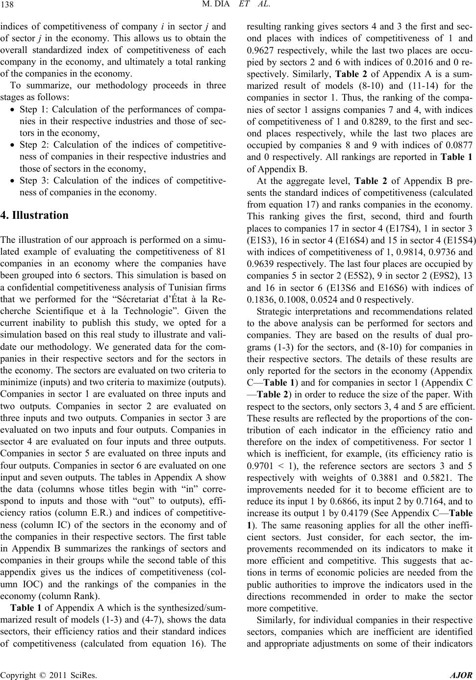

138 M. DIA ET AL.
indices of competitiveness of company i in sector j and
of sector j in the economy. This allows us to obtain the
overall standardized index of competitiveness of each
company in the economy, and ultimately a total ranking
of the companies in the economy.
To summarize, our methodology proceeds in three
stages as follows:
 Step 1: Calculation of the performances of compa-
nies in their respective industries and those of sec-
tors in the economy,
 Step 2: Calculation of the indices of competitive-
ness of companies in their respective industries and
those of sectors in the economy,
 Step 3: Calculation of the indices of competitive-
ness of companies in the economy.
4. Illustration
The illustration of our approach is performed on a simu-
lated example of evaluating the competitiveness of 81
companies in an economy where the companies have
been grouped into 6 sectors. This simulation is based on
a confidential competitiveness analysis of Tunisian firms
that we performed for the “Sécretariat d’État à la Re-
cherche Scientifique et à la Technologie”. Given the
current inability to publish this study, we opted for a
simulation based on this real study to illustrate and vali-
date our methodology. We generated data for the com-
panies in their respective sectors and for the sectors in
the economy. The sectors are evaluated on two criteria to
minimize (inputs) and two criteria to maximize (outputs).
Companies in sector 1 are evaluated on three inputs and
two outputs. Companies in sector 2 are evaluated on
three inputs and two outputs. Companies in sector 3 are
evaluated on two inputs and four outputs. Companies in
sector 4 are evaluated on four inputs and three outputs.
Companies in sector 5 are evaluated on three inputs and
four outputs. Companies in sector 6 are evaluated on one
input and seven outputs. The tables in Appendix A show
the data (columns whose titles begin with “in” corre-
spond to inputs and those with “out” to outputs), effi-
ciency ratios (column E.R.) and indices of competitive-
ness (column IC) of the sectors in the economy and of
the companies in their respective sectors. The first table
in Appendix B summarizes the rankings of sectors and
companies in their groups while the second table of this
appendix gives us the indices of competitiveness (col-
umn IOC) and the rankings of the companies in the
economy (column Rank).
Table 1 of Appendix A which is the synthesized/sum-
marized result of models (1-3) and (4-7), shows the data
sectors, their efficiency ratios and their standard indices
of competitiveness (calculated from equation 16). The
resulting ranking gives sectors 4 and 3 the first and sec-
ond places with indices of competitiveness of 1 and
0.9627 respectively, while the last two places are occu-
pied by sectors 2 and 6 with indices of 0.2016 and 0 re-
spectively. Similarly, Table 2 of Appendix A is a sum-
marized result of models (8-10) and (11-14) for the
companies in sector 1. Thus, the ranking of the compa-
nies of sector 1 assigns companies 7 and 4, with indices
of competitiveness of 1 and 0.8289, to the first and sec-
ond places respectively, while the last two places are
occupied by companies 8 and 9 with indices of 0.0877
and 0 respectively. All rankings are reported in Table 1
of Appendix B.
At the aggregate level, Table 2 of Appendix B pre-
sents the standard indices of competitiveness (calculated
from equation 17) and ranks companies in the economy.
This ranking gives the first, second, third and fourth
places to companies 17 in sector 4 (E17S4), 1 in sector 3
(E1S3), 16 in sector 4 (E16S4) and 15 in sector 4 (E15S4)
with indices of competitiveness of 1, 0.9814, 0.9736 and
0.9639 respectively. The last four places are occupied by
companies 5 in sector 2 (E5S2), 9 in sector 2 (E9S2), 13
and 16 in sector 6 (E13S6 and E16S6) with indices of
0.1836, 0.1008, 0.0524 and 0 respectively.
Strategic interpretations and recommendations related
to the above analysis can be performed for sectors and
companies. They are based on the results of dual pro-
grams (1-3) for the sectors, and (8-10) for companies in
their respective sectors. The details of these results are
only reported for the sectors in the economy (Appendix
C—Table 1) and for companies in sector 1 (Appendix C
—Table 2) in order to reduce the size of the paper. With
respect to the sectors, only sectors 3, 4 and 5 are efficient.
These results are reflected by the proportions of the con-
tribution of each indicator in the efficiency ratio and
therefore on the index of competitiveness. For sector 1
which is inefficient, for example, (its efficiency ratio is
0.9701 < 1), the reference sectors are sectors 3 and 5
respectively with weights of 0.3881 and 0.5821. The
improvements needed for it to become efficient are to
reduce its input 1 by 0.6866, its inpu t 2 by 0.7164 , and to
increase its output 1 by 0.4179 (See Appendix C—Table
1). The same reasoning applies for all the other ineffi-
cient sectors. Just consider, for each sector, the im-
provements recommended on its indicators to make it
more efficient and competitive. This suggests that ac-
tions in terms of economic policies are needed from the
public authorities to improve the indicators used in the
directions recommended in order to make the sector
more competitive.
Similarly, for individual companies in their respective
sectors, companies which are inefficient are identified
and appropriate adjustments on some of their indicators

M. DIA ET AL.
139
are recommended based on their units of reference. For
sector 1, companies 4, 6, 7 and 10 are efficient, and all
others are inefficient. In this case, company 1 of sector 1
has an efficiency ratio of 0.8466 (<1) and its benchmark
companies are companies 4, 6 and 7 respectively with
weights 0.5174, 0.3885 and 0.0573. The improvements
needed for it to become efficient in its sector are to re-
duce its inpu t 1 by 1.5357, its in put 2 by 0.1 227, its inpu t
3 by 92.0246 and not to increase its two outputs ((See
Appendix C—Table 2)). This suggests that management
and planning actions are needed to improve the indica-
tors used in the directions recommended in order to make
the company more competitive.
Regarding now the improvements of the companies in
the economy, we consider both the improvements of the
companies in their sectors as well as those of the sectors
in the economy. For company 1 of sector 1 to become
efficient and more competitive in the economy, not only
it must be adjusted in its sector, but its sector must also
be adjusted in the economy. The optimal improvements
for this company to become efficient are to reduce, in
sector 1, its input 1 by 1.5357, its input 2 by 0.1227, its
input 3 by 92.02 46 and n ot to increase its two outputs. In
addition, its sector must reduce, in the economy, its input
1 by 0.6866 and its input 2 by 0.7164 while in creasin g its
output 1 by 0.4179. The same reasoning applies for all
the other companies in the economy. Companies that are
efficient in their sectors, and whose sectors are efficient
in the economy do not require any specific improve-
ments, but only some monitoring. Companies that fall
into this category ar e companies 1, 3, 4, 8, 9, 10, 11 , 12,
13 and 14 of sector 3, companies 2, 5, 7, 9, 10, 11, 15, 16
and 17 of sector 4, and companies 1, 2, 3, 4, 6 and 7 of
sector 5.
In order to explain or justify the level of competitive-
ness of a company i belonging to a given sector j (EiSj),
one should adopt the same considerations as in the pre-
vious analysis by addressing the competitiveness of the
sector j in the economy and the competitiveness of com-
pany i in its sector. For example, if EiSj is weakly com-
petitive at the global level, the reasons for this weakness
in terms of competitiveness analysis can be explained or
justified by the following: 1) the low level of competi-
tiveness of company i in its sector and, in this case, deci-
sion-makers must take the necessary steps to bring its
competitiveness to the same level as the competitive
companies in its sector (Sj); 2) the low level of competi-
tiveness of the sector j in the economy wh ere, in this c as e,
the company generally has no control or influence on the
indicators of the competitiveness of the sector; however,
it is to be noted that if this stud y was spon sored or super-
vised by public administration, authorities could then
take the necessary actions (economic and trade policies)
to improve the competitiveness of sector j and therefore
this will be reflected on the competitiveness of EiSj in th e
economy; or 3) both scenarios may apply.
5. Conclusions
In this paper, we proposed a new methodology for
evaluating hierarchical performance that we illustrated
through a simulated case. Our methodology takes into
account the heterogeneity of the companies to be com-
pared. It suggests a tree structure form with two group-
ings (economy and sectors) in order to better identify and
define the appropriate indicators of competitiveness. It
calculates for each grouping level the performance ratios
by using the DEA technique. In each grouping level, we
also determined the indices of competitiveness of the
compared units (companies and sectors). We have also
proposed a combination of two grouping levels of per-
formance to infer the performances and indices of com-
petitiveness in the economy. Finally, the case studied and
the results obtained demonstrate the applicability of the
proposed methodology.
The approach developed here refers only to a case of
evaluating companies in an economy using a single level
of grouping through economic activity sectors. However,
our approach, with the conceptual framework described
here, could also be used in other areas. For example, it
could be applied to a comparison of the competitiveness
of globalized companies taking into account their affilia-
tions to given countries, sub-regions, or economic spaces
and providing new ways for grouping on several levels,
where at each level several comparison indicators could
be considered. Furthermore, as most economic and social
information is by nature generally ambiguous, uncertain
or unclear, it is also important to extend the competi-
tiveness measure to the fuzzy context.
6. References
[1] O. Kettani, F. Ben Abdelaziz and M. Dia, “Méthodologie
Multicritère Pour la Sélection de Projets d'Investissement
en Tunisie,” In: M. Oral and O. Kettani, Eds., Globalisa-
tion and Competitiveness: Implications for Policy and
Strategy Formulation, Bilkent University Press, Bilkent,
1997, pp. 381-396.
[2] A. Charnes, W. W. Cooper and E. Rhodes, “Measuring
the Efficiency of Decision-Making Units,” European Jour-
nal of Operational Research, Vol. 2, No. 6, 1978, pp.
429-444. doi:10.1016/0377-2217(78)90138-8
[3] R. D. Banker, “Productivity Measurement and Manage-
ment Control,” In: P. Kleindorfer, Ed., Management of
Productivity and Technology in Manufacturing, Plenum
Press, New York, 1985, pp. 239-257.
doi:10.1007/978-1-4613-2507-9_10

M. DIA ET AL.
140
[4] M. Oral and H. Chabchoub, “On the Methodology of
World Competitiveness Report,” European Journal of
Operational Research, Vol. 90, No. 3, 1996, pp. 514-535.
doi:10.1016/0377-2217(94)00370-X
[5] M. Oral, O. Kettani and P. Lang, “A Methodology for
Collective Evaluation and Selection of Industrial R&D
Projects,” Management Science, Vol. 37, No. 7, 1991, pp.
871-885. doi:10.1287/mnsc.37.7.871
[6] K. K. Sinha, “Moving Frontier Analysis: An Application
of Data Envelopment Analysis for Competitive Analysis
of a High-Technology Manufacturing Plant,” Annals of
Operations Research, Vol. 66, No. 3, 1996, pp. 197-218.
doi:10.1007/BF02187591
[7] M. Oral and O. Kettani, Eds., “Globalisation and Com-
petitiveness: Implications for Policy and Strategy Formu-
lation,” Bilkent University Press, Bilkent, 1997.
[8] M. E. Porter, “The Competitive Advantage of Nations,”
Harvard Business Review, Vol. 68, N o. 2, 1990, pp. 73-93.
[9] M. E. Porter, Ed., “Competition in Global Industries,”
Harvard Business School Press, Boston, 1986.
[10] D. G. McFetridge, “La Compétitivité: Notions et Mesures,”
Document Hors-Série Numé ro 5, Industrie Canada , Ottawa,
1995, pp. 1-45.
[11] M. E. Porter, “Competitive Advantage: Creating and Sus-
taining Superior Performance,” Free Press, New York,
1985.
[12] M. Oral, “A Methodology for Competitiveness Analysis
and Strategy Formulation in Glass Industry,” European
Journal of Operational Research, Vol. 68, No. 1, 1993,
pp. 9-22. doi:10.1016/0377-2217(93)90074-W
[13] L. Castelli, R. Pesenti and W. Ukovich, “A Classification
of DEA Models When the Internal Structure of the Deci-
sion Making Units Is Considered,” Annals of Operations
Research, Vol. 173, No. 1, 2010, pp. 207-235.
doi:10.1007/s10479-008-0414-2
[14] W. D. Cook and R. H. Green, “Evaluating Power Plant
Efficiency: A Hierarchical Model,” Computers & Opera-
tions Research, Vol. 32, No. 4, 2005, pp. 813-823.
doi:10.1016/j.cor.2003.08.019
[15] L. Castelli, R. Pesenti and W. Ukovich, “DEA-Like Mod-
els for the Efficiency Evaluation of Hierarchically Struc-
tured Units,” European Journal of Operational Research,
Vol. 154, No. 2, 2004, pp. 465-476.
doi:10.1016/S0377-2217(03)00182-6
[16] W. D. Cook, D. Chai, J. Doyle and R. Green, “Hierarchie s
and Groups in DEA,” Journal of Productivity Analysis,
Vol. 10, No. 2, 1998, pp. 177-198.
doi:10.1023/A:1018625424184
[17] T. R. Sexton, R. H. Silkman and A. J. Hogan, “Data En-
velopment Analysis: Critique and Extensions,” In: R. H.
Silkman, Ed., Measuring Efficiency: An Assessment of
Data Envelopment Analysis, Jossey-Bass, San Francisco,
1986.
[18] J. Doyle and R. Green, “Efficiency and Cross-Efficiency
in DEA: Derivations, Meanings and Uses,” Journal of
Operational Research and Society, Vol. 45, No. 5, 1994,
pp. 567-578.
[19] A. Charnes and W. W. Cooper, “Programming with Lin-
ear Fractional Functional,” Naval Research Logistics
Quarterly, Vol. 9, No. 3-4, 1962, pp. 181-185.
doi:10.1002/nav.3800090303
[20] R. D. Banker, A. Charnes and W. W. Cooper, “Some
Models for Estimating Technical and Scale Efficiencies
in Data Envelopment Analysis,” Management Science,
Vol. 30, No. 9, 1984, pp. 1078-1092.
doi:10.1287/mnsc.30.9.1078
[21] G. Yu, Q. Wei and P. Brockett, “A Generalized Data
Envelopment Analysis Model: A Unification and Exten-
sion of Existing Methods for Efficiency Analysis of De-
cision Making Units,” Annals of Operations Research,
Vol. 66, 1996, pp. 47-89.
[22] Y.-M. Wang and K.-S. Chin, “Some Alternative Models
for DEA Cross-Efficiency Evaluation,” International
Journal of Production Economics, Vol. 128, No. 1, 2010,
pp. 332-338. doi:10.1016/j.ijpe.2010.07.032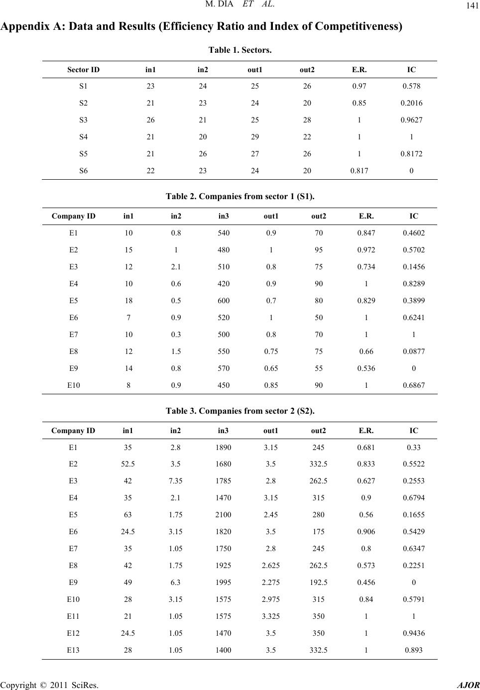

M. DIA ET AL.
141
Appendix A: Data and Results (Efficiency Ratio and Index of Competitiveness)
Table 1. Sectors.
Sector ID in1 in2 out1 out2 E.R. IC
S1 23 24 25 26 0.97 0.578
S2 21 23 24 20 0.85 0.2016
S3 26 21 25 28 1 0.9627
S4 21 20 29 22 1 1
S5 21 26 27 26 1 0.8172
S6 22 23 24 20 0.817 0
Table 2. Companies from sector 1 (S1).
Company ID in1 in2 in3 out1 out2 E.R. IC
E1 10 0.8 540 0.9 70 0.847 0.4602
E2 15 1 480 1 95 0.972 0.5702
E3 12 2.1 510 0.8 75 0.734 0.1456
E4 10 0.6 420 0.9 90 1 0.8289
E5 18 0.5 600 0.7 80 0.829 0.3899
E6 7 0.9 520 1 50 1 0.6241
E7 10 0.3 500 0.8 70 1 1
E8 12 1.5 550 0.75 75 0.66 0.0877
E9 14 0.8 570 0.65 55 0.536 0
E10 8 0.9 450 0.85 90 1 0.6867
Table 3. Companies from sector 2 (S2).
Company ID in1 in2 in3 out1 out2 E.R. IC
E1 35 2.8 1890 3.15 245 0.681 0.33
E2 52.5 3.5 1680 3.5 332.5 0.833 0.5522
E3 42 7.35 1785 2.8 262.5 0.627 0.2553
E4 35 2.1 1470 3.15 315 0.9 0.6794
E5 63 1.75 2100 2.45 280 0.56 0.1655
E6 24.5 3.15 1820 3.5 175 0.906 0.5429
E7 35 1.05 1750 2.8 245 0.8 0.6347
E8 42 1.75 1925 2.625 262.5 0.573 0.2251
E9 49 6.3 1995 2.275 192.5 0.456 0
E10 28 3.15 1575 2.975 315 0.84 0.5791
E11 21 1.05 1575 3.325 350 1 1
E12 24.5 1.05 1470 3.5 350 1 0.9436
E13 28 1.05 1400 3.5 332.5 1 0.893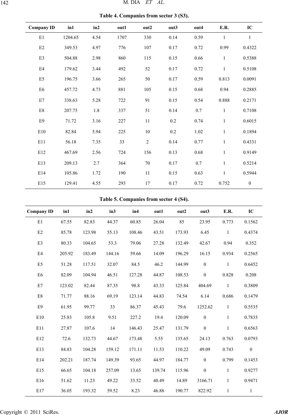

142 M. DIA ET AL.
Table 4. Companies from sector 3 (S3).
Company ID in1 in2 out1 out2 out3 out4 E.R. IC
E1 1204.65 4.54 1707 330 0.14 0.59 1 1
E2 349.53 4.97 776 107 0.17 0.72 0.99 0.4322
E3 504.88 2.98 860 115 0.15 0.66 1 0.5388
E4 179.62 3.44 492 52 0.17 0.72 1 0.5108
E5 196.75 3.66 265 50 0.17 0.59 0.813 0.0091
E6 457.72 4.73 881 105 0.15 0.68 0.94 0.2885
E7 338.63 5.28 722 91 0.15 0.54 0.888 0.2171
E8 207.75 1.8 337 51 0.14 0.7 1 0.7108
E9 71.72 3.16 227 11 0.2 0.74 1 0.6015
E10 82.84 5.94 225 10 0.2 1.02 1 0.1894
E11 56.18 7.35 33 2 0.14 0.77 1 0.4331
E12 467.69 2.56 724 156 0.13 0.68 1 0.9149
E13 209.13 2.7 364 70 0.17 0.7 1 0.5214
E14 105.86 1.72 190 11 0.15 0.63 1 0.5944
E15 129.41 4.55 293 17 0.17 0.72 0.752 0
Table 5. Companies from sector 4 (S4).
Company ID in1 in2 in3 in4 out1 out2 out3 E.R. IC
E1 67.55 82.83 44.37 60.85 26.04 85 23.95 0.773 0.1562
E2 85.78 123.98 55.13 108.46 43.51 173.93 6.45 1 0.4374
E3 80.33 104.65 53.3 79.06 27.28 132.49 42.67 0.94 0.352
E4 205.92 183.49 144.16 59.66 14.09 196.29 16.15 0.934 0.2565
E5 51.28 117.51 32.07 84.5 46.2 144.99 0 1 0.6452
E6 82.09 104.94 46.51 127.28 44.87 108.53 0 0.828 0.208
E7 123.02 82.44 87.35 98.8 43.33 125.84 404.69 1 0.3809
E8 71.77 88.16 69.19 123.14 44.83 74.54 6.14 0.686 0.1479
E9 61.95 99.77 33 86.37 45.43 79.6 1252.62 1 0.5535
E10 25.83 105.8 9.51 227.2 19.4 120.09 0 1 0.7835
E11 27.87 107.6 14 146.43 25.47 131.79 0 1 0.6563
E12 72.6 132.73 44.67 173.48 5.55 135.65 24.13 0.763 0.0793
E13 84.83 104.28 159.12 171.11 11.53 110.22 49.09 0.743 0
E14 202.21 187.74 149.39 93.65 44.97 184.77 0 0.799 0.1453
E15 66.65 104.18 257.09 13.65 139.74 115.96 0 1 0.9277
E16 51.62 11.23 49.22 33.52 40.49 14.89 3166.711 0.9471
E17 36.05 193.32 59.52 8.23 46.88 190.77 822.92 1 1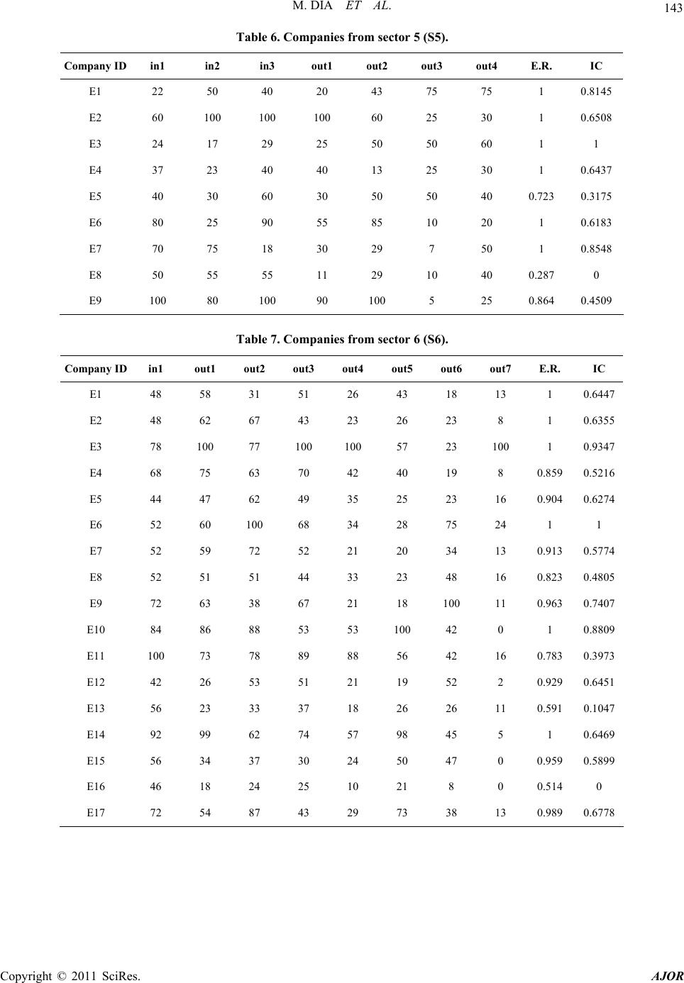

M. DIA ET AL.
143
Table 6. Companies from sector 5 (S5).
Company ID in1 in2 in3 out1 out2 out3 out4 E.R. IC
E1 22 50 40 20 43 75 75 1 0.8145
E2 60 100 100 100 60 25 30 1 0.6508
E3 24 17 29 25 50 50 60 1 1
E4 37 23 40 40 13 25 30 1 0.6437
E5 40 30 60 30 50 50 40 0.723 0.3175
E6 80 25 90 55 85 10 20 1 0.6183
E7 70 75 18 30 29 7 50 1 0.8548
E8 50 55 55 11 29 10 40 0.287 0
E9 100 80 100 90 100 5 25 0.864 0.4509
Table 7. Companies from sector 6 (S6).
Company ID in1 out1 out2 out3 out4 out5 out6 out7 E.R. IC
E1 48 58 31 51 26 43 18 13 1 0.6447
E2 48 62 67 43 23 26 23 8 1 0.6355
E3 78 100 77 100 100 57 23 100 1 0.9347
E4 68 75 63 70 42 40 19 8 0.859 0.5216
E5 44 47 62 49 35 25 23 16 0.904 0.6274
E6 52 60 100 68 34 28 75 24 1 1
E7 52 59 72 52 21 20 34 13 0.913 0.5774
E8 52 51 51 44 33 23 48 16 0.823 0.4805
E9 72 63 38 67 21 18 100 11 0.963 0.7407
E10 84 86 88 53 53 100 42 0 1 0.8809
E11 100 73 78 89 88 56 42 16 0.783 0.3973
E12 42 26 53 51 21 19 52 2 0.929 0.6451
E13 56 23 33 37 18 26 26 11 0.591 0.1047
E14 92 99 62 74 57 98 45 5 1 0.6469
E15 56 34 37 30 24 50 47 0 0.959 0.5899
E16 46 18 24 25 10 21 8 0 0.514 0
E17 72 54 87 43 29 73 38 13 0.989 0.6778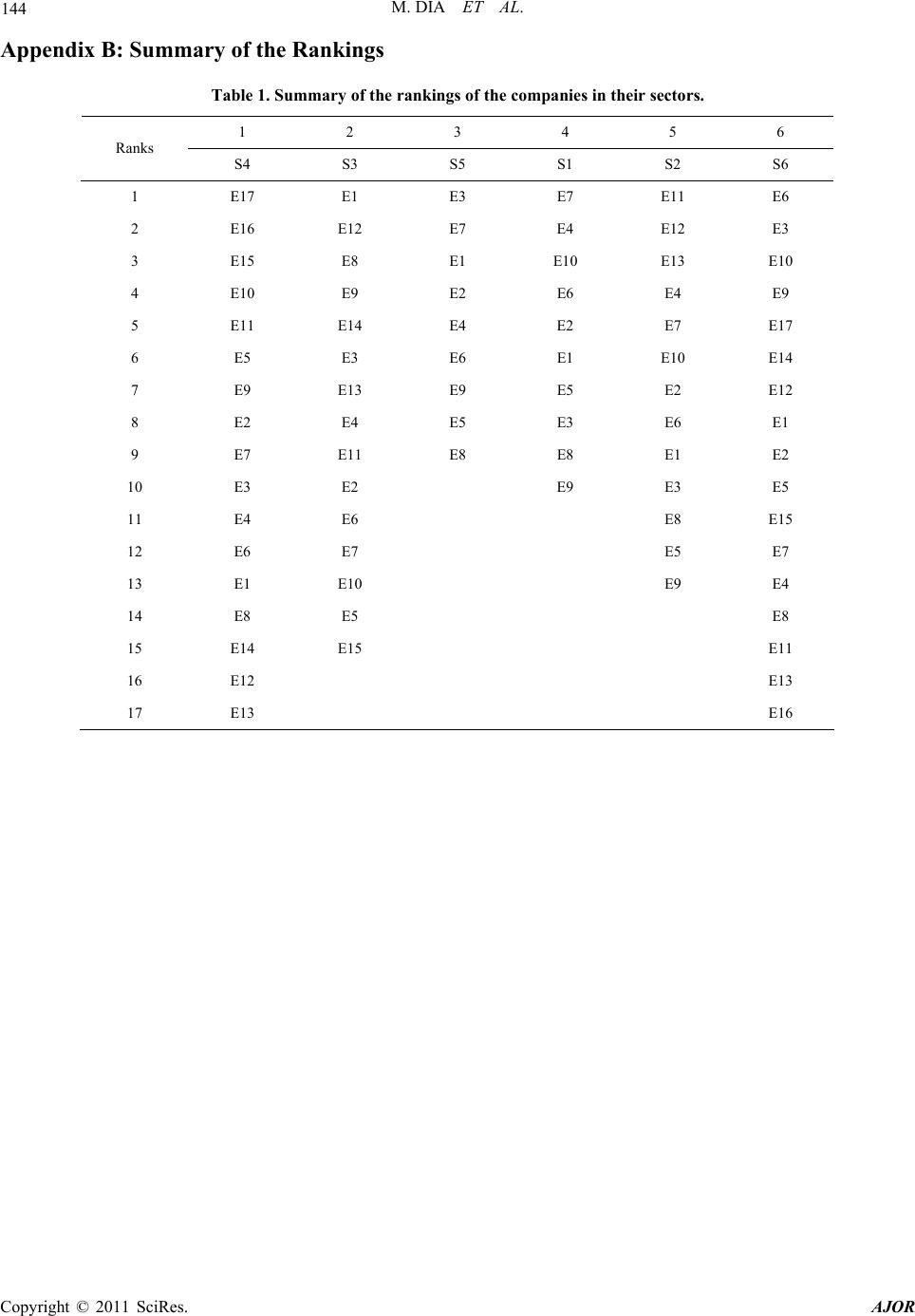

144 M. DIA ET AL.
Appendix B: Summary of the Rankings
Table 1. Summary of the rankings of the companies in their sectors.
1 2 3 4 5 6
Ranks S4 S3 S5 S1 S2 S6
1 E17 E1 E3 E7 E11 E6
2 E16 E12 E7 E4 E12 E3
3 E15 E8 E1 E10 E13 E10
4 E10 E9 E2 E6 E4 E9
5 E11 E14 E4 E2 E7 E17
6 E5 E3 E6 E1 E10 E14
7 E9 E13 E9 E5 E2 E12
8 E2 E4 E5 E3 E6 E1
9 E7 E11 E8 E8 E1 E2
10 E3 E2 E9 E3 E5
11 E4 E6 E8 E15
12 E6 E7 E5 E7
13 E1 E10 E9 E4
14 E8 E5 E8
15 E14 E15 E11
16 E12 E13
17 E13 E16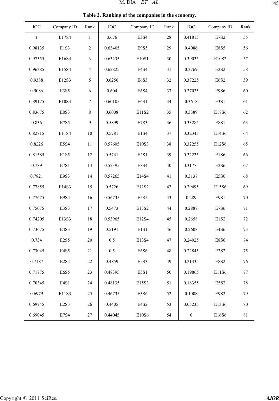

M. DIA ET AL.
145
Table 2. Ranking of the companies in the economy.
IOC Company ID Rank IOC Company ID RankIOC Company ID Rank
1 E17S4 1 0.676 E3S4 28 0.41815 E7S2 55
0.98135 E1S3 2 0.63405 E9S5 29 0.4086 E8S5 56
0.97355 E16S4 3 0.63235 E10S1 30 0.39035 E10S2 57
0.96385 E15S4 4 0.62825 E4S4 31 0.3769 E2S2 58
0.9388 E12S3 5 0.6256 E6S3 32 0.37225 E6S2 59
0.9086 E3S5 6 0.604 E6S4 33 0.37035 E9S6 60
0.89175 E10S4 7 0.60105 E6S1 34 0.3618 E3S1 61
0.83675 E8S3 8 0.6008 E11S2 35 0.3389 E17S6 62
0.836 E7S5 9 0.5899 E7S3 36 0.33285 E8S1 63
0.82815 E11S4 10 0.5781 E1S4 37 0.32345 E14S6 64
0.8226 E5S4 11 0.57605 E10S3 38 0.32255 E12S6 65
0.81585 E1S5 12 0.5741 E2S1 39 0.32235 E1S6 66
0.789 E7S1 13 0.57395 E8S4 40 0.31775 E2S6 67
0.7821 E9S3 14 0.57265 E14S4 41 0.3137 E5S6 68
0.77855 E14S3 15 0.5726 E12S2 42 0.29495 E15S6 69
0.77675 E9S4 16 0.56735 E5S5 43 0.289 E9S1 70
0.75075 E3S3 17 0.5473 E13S2 44 0.2887 E7S6 71
0.74205 E13S3 18 0.53965 E12S4 45 0.2658 E1S2 72
0.73675 E4S3 19 0.5191 E1S1 46 0.2608 E4S6 73
0.734 E2S5 20 0.5 E13S4 47 0.24025 E8S6 74
0.73045 E4S5 21 0.5 E6S6 48 0.22845 E3S2 75
0.7187 E2S4 22 0.4859 E5S3 49 0.21335 E8S2 76
0.71775 E6S5 23 0.48395 E5S1 50 0.19865 E11S6 77
0.70345 E4S1 24 0.48135 E15S3 51 0.18355 E5S2 78
0.6979 E11S3 25 0.46735 E3S6 52 0.1008 E9S2 79
0.69745 E2S3 26 0.4405 E4S2 53 0.05235 E13S6 80
0.69045 E7S4 27 0.44045 E10S6 54 0 E16S6 81

M. DIA ET AL.
146
Appendix C: Improvement Opportunities
Table 1. Improvement opportunities for the sectors in the economy.
Sector ID in1 in2 out1 out2
S1 –0.6866 –0.7164 0.4179 0
S2 –3.15 –4.05 0 0
S6 –4.0369 –4.2204 0 0
Table 2. Improvement opportunities for the companies in their sector 1.
Company ID in1 in2 in3 out1 out2
E1 –1.5337 –0.1227 –92.0246 0 0
E2 –3.8889 –0.3333 –13.3333 0 5
E3 –3.1912 –1.5621 –135.6273 0 4.0256
E5 –7.5238 –0.0857 –102.8571 0.1714 0
E8 –4.0791 –0.9207 –186.9596 0 0
E9 –6.7572 –0.371 –264.3243 0 9.8151
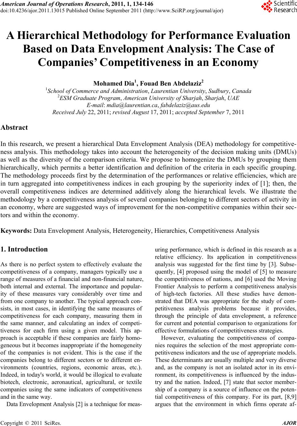