American Journal of Oper ations Research, 2011, 1, 118-133
doi:10.4236/ajor.2011.13014 Published Online September 2011 (http://www.SciRP.org/journal/ajor)
Solving the Multi Observer 3D Visual Area Coverage
Scheduling Problem by Decomposition
Helman I. Stern1, Moshe Zofi1,2, Moshe Kaspi1
1Department of Ind ust ri al E n g i neeri n g an d Ma na gement,
Ben Gurion University of the Negev, Beer-Sheva, Israel
2Department of Industrial Management, Sapir College, Sderot, Israel
Received April 26, 2011; revised May 15, 2011; accepted June 11, 2011
Abstract
This paper presents two solution methodologies for the Visual Area Coverage Scheduling problem. The ob-
jective is to schedule a number of dynamic observers over a given 3D terrain such that the total visual area
covered (viewed) over a planning horizon is maximal. This problem is a more complicated extension of the
Set Covering Problem, known to be Np-Hard. We present two decomposition based heuristic methods each
containing three stages. The first methodology finds a set of area covering points, and then partitions them
into routes (cover first, partition second). The second methodology partitions the area into a region for each
observer, and then finds the best covering points and routes (partition first, cover second). In each, a last
stage determines dwell (view) times so as to maximize the visible coverage smoothly over the terrain. Com-
parative tests were made for the two methods on real terrains for several scenarios. When comparing the best
solutions of both methods the CF-PS method was slightly better. However, because of the increased compu-
tation time we suggest that the PF-CS method with a fine terrain approximation be used. This method is
faster as partitioning the terrain into separate regions for each observer results in smaller coverage and rout-
ing problems. A sensitivity analysis of the number of observation points to the total number of terrain points
covered depicted the classical notion of decreasing returns to scale, increasing in a convex manner as the
number of observation points was increased. The best method achieved 100 percent coverage of the terrain
by using only 2.7 percent of its points as observation points. Experts stated that the computer based solutions
can save precious time and help plan observation missions with satisfying results.
Keywords: Heuristic Search, Genetic Algorithm, Computer Vision, Multi Agents, Meta-Heuristic
1. Introduction
The development of Geographical Information Systems
(GIS) in recent years has made a large contribution to the
ability to solve various terrain related problems effi-
ciently. Problems such as; 1) finding the optimal path
between two points over a rough terrain, and 2) locating
observers in order to visually cover an area can now be
solved using mathematical tools. Locating observers over
a given area can be modeled as the Set Covering Prob-
lem (SCP). The traditional art gallery problem first pro-
posed by Chvatal deals with the problem of finding the
minimal number of observers required for complete visual
coverage of a 2D polygon [1]. This problem is NP-hard,
with popular approximations running in [2].
The approach does not model dynamic observers, the
quality of coverage, nor does it consider costs.

logOn n
The Visual Area Coverage Scheduling (VACS) prob-
lem offered here combines the two problems of; locating
observation points over a 3D terrain, and routing multi-
ple observers through them. Creating the best synchro-
nization between the observers so as to view the maximal
area of the terrain is the main objective. A second objec-
tive is to smooth coverage over the terrain. The VACS
problem has been formulated and solved using a Genetic
Algorithm in [3,4]. This paper introduces two decompo-
sition based methodologies; 1) cover first, partition sec-
ond (CF-PS) and 2) partition first, cover second (PF-CS),
each containing three stages. The analysis is divided into
finding observation points, routing observers through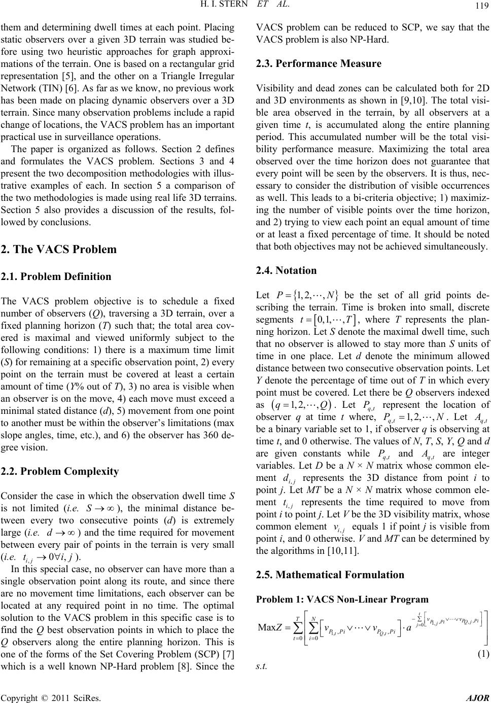

H. I. STERN ET AL.
119
them and determining dwell times at each point. Placing
static observers over a given 3D terrain was studied be-
fore using two heuristic approaches for graph approxi-
mations of the terrain. One is based on a rectangular grid
representation [5], and the other on a Triangle Irregular
Network (TIN) [6]. As far as we know, no previous work
has been made on placing dynamic observers over a 3D
terrain. Since many observation problems include a rapid
change of locations, the VACS problem has an important
practical use in surveillance operations.
The paper is organized as follows. Section 2 defines
and formulates the VACS problem. Sections 3 and 4
present the two decomposition methodologies with illus-
trative examples of each. In section 5 a comparison of
the two methodologies is made using real life 3D terrains.
Section 5 also provides a discussion of the results, fol-
lowed by conclusions.
2. The VACS Problem
2.1. Problem Definition
The VACS problem objective is to schedule a fixed
number of observers (Q), traversing a 3D terrain, over a
fixed planning horizon (T) such that; the total area cov-
ered is maximal and viewed uniformly subject to the
following conditions: 1) there is a maximum time limit
(S) for remaining at a specific observation point, 2) every
point on the terrain must be covered at least a certain
amount of time (Y% out of T), 3) no area is visible when
an observer is on the move, 4) each move must exceed a
minimal stated distance (d), 5) movement from one point
to another must be within the observer’s limitations (max
slope angles, time, etc.), and 6) the observer has 360 de-
gree vision.
2.2. Problem Complexity
Consider the case in which the observation dwell time S
is not limited (i.e. ), the minimal distance be-
tween every two consecutive points (d) is extremely
large (i.e. ) and the time required for movement
between every pair of points in the terrain is very small
(i.e. ).
S
j
d
0,ti
,ij
In this special case, no observer can have more than a
single observation point along its route, and since there
are no movement time limitations, each observer can be
located at any required point in no time. The optimal
solution to the VACS problem in this specific case is to
find the Q best observation points in which to place the
Q observers along the entire planning horizon. This is
one of the forms of the Set Covering Problem (SCP) [7]
which is a well known NP-Hard problem [8]. Since the
VACS problem can be reduced to SCP, we say that the
VACS problem is also NP-Hard.
2.3. Performance Measure
Visibility and dead zones can be calculated both for 2D
and 3D environments as shown in [9,10]. The total visi-
ble area observed in the terrain, by all observers at a
given time t, is accumulated along the entire planning
period. This accumulated number will be the total visi-
bility performance measure. Maximizing the total area
observed over the time horizon does not guarantee that
every point will be seen by the observers. It is thus, nec-
essary to consider the distribution of visible occurrences
as well. This leads to a bi-criteria objective; 1) maximiz-
ing the number of visible points over the time horizon,
and 2) trying to view each point an equal amount of time
or at least a fixed percentage of time. It should be noted
that both objectives may not be achieved simultaneously.
2.4. Notation
Let


1, 2,,PN be the set of all grid points de-
scribing the terrain. Time is broken into small, discrete
segments


0,1,t,T, where T represents the plan-
ning horizon. Let S denote the maximal dwell time, such
that no observer is allowed to stay more than S units of
time in one place. Let d denote the minimum allowed
distance between two consecutive observation points. Let
Y denote the percentage of time out of T in which every
point must be covered. Let there be Q observers indexed
as


1, 2,,qQ. Let represent the location of
observer q at time t wher,N. L,qt
,qt
P
e, 1, 2,,
qt
Pet
A
be a binary variable set to 1, if observer q is observing at
time t, and 0 otherwise. The values of N, T, S, Y, Q and d
are given constants while ,qt and ,qt P
A
are integer
variables. Let D be a N × N matrix whose common ele-
ment ,ij represents the 3D distance from point i to
point j. Let MT be a N × N matrix whose common ele-
ment ,ij represents the time required to move from
point i to point j. Let V be the 3D visibility matrix, whose
common element ,ij equals 1 if point j is visible from
point i, and 0 otherwise. V and MT can be determined by
the algorithms in [10,11].
d
t
v
2.5. Mathematical Formulation
Problem 1: VACS Non-Linear Program
,
,,
1,
0
1, ,
,,
00
Max
t
PPi
PPi Qj
j
j
tQt
vv
TN
PPiP Pi
ti
Zvva

















 

(1)
s.t.

120 H. I. STERN ET AL.
1
,0; ,
tS
qt
t
A
qt
 
 (2)

,, ,, ,
,1
0, ,1,0, ,
qt qm
P Pqtqmqk
tkm
ddAA A
tmmT


 


0;, q
qt
i

(3)
 ,,1
,1; ,
qt qt
PP
t

(4)
1, 2,,
,, ,
0
0;
tt Qt
T
PPiPPiP Pi
t
vvv YT


 

 (5)
where ,
,0,1 qt
A,1, ,
qt
P
N
, ,
1, ,qQ0, ,tT

,
. 1a
The objective function Z in (1) represents the penal-
ized total visibility throughout the entire planning hori-
zon. The OR logic function returns the value of 1, if at
least one of the Q observers sees point i at time t. This
term is multiplied by an exponential function which de-
creases according to the number of previous times the
point was viewed. This smoothes out the visibility over
all the points by insuring the more times a point has been
viewed up to time t, the less value there is to view it
again. Constraint (2) prevents an observer from staying
in an observation point more than S continuous segments
of time. Constraint (3) insures a distance of at least d
when a move occurs. Constraint (4) is added to avoid
non feasible solutions in which the observer moves to a
point that is not adjacent to its current location in the first
step of its path to the next observation point. Constraint
(5) ensures that every point will be seen Y percent of the
time. A more detailed explanation for this formulation
can be found in [3]. This formulation is untenable using
mathematical programming techniques as it contains
logical and nonlinear expressions in both its objective
function and constraints. Hence, two heuristic solution
approaches are proffered in the next two sections
3. The Cover First, Partition Second
(CF-PS) Heuristic
3.1. Overview
This methodology has three phases. The first phase se-
lects M specific locations in the terrain to be visited by
the observers. The number of observation points is fixed
at
M
QK, where each observer will stop at K ob-
servation points. Four alternative covering heuristics are
developed for this purpose, which are described in the
next section. The second phase solves a modified Vehi-
cle Routing Problem (VRP) [12] heuristic to iteratively
combine points until there are Q routes, one for each
observer. The observation time at each point along every
route is determined using linear programming in the third
Figure 1. Flow chart of CF-PS methodology.
phase. Figure 1 provides a flowchart of steps of the
CF-PS procedure.
3.2. Phase I—Finding M Preferred
Observation Points
This problem is a special case of the SCP which is
known as NP-hard. There are many covering heuristics
for finding the best M locations to place static observers
(SCP heuristics). We considered four different covering
heuristics referred to as: 1) COVER1, 2) COVER2, 3)
COVERGA, and 4) COVERTIN. Each in turn is ex-
plained below.
3.2.1. COVER1— Covering Heuristic 1
COVER1 uses a greedy search, starting at the point with
the largest cover, while covering continues to the next
points, which will increase the total viewable area. Let
represent the subset of points visible to i. Let
i
VPP
i
V represent the number of points within the subset i.
Let
V
A
P represent the subset of preferred observation
points. The objective of the heuristic is to find
A
M
a tosuch that the total visible are A: will
maximized. lgorithm
int findOrder the
po
i
i
PA
V

be
COVER1 A
Step 1: For every poi PP i V.
ints in a descending order according to i V and start-
ing from the top.
Step 2: Start with the current point . Add to A
an
i
Pi P
d delete it from the list. Go over the list of points and
update i V for every point
j
P such that
j
ji
VVV

.
Reorder the list according to
j
V.

H. I. STERN ET AL.
121
po . If Step 3: Find the current int i P0
i
V and
A
M repeat step 2. Else, return A.
.2.2. COVER2—Covering Heuristic 2
d continues to
m
int findOrder the
po
3
COVER2 starts with the greedy search an
the next best point, which is not visible from the previous
selected points [5,6].
COVER2 Algorith
Step 1: For every poi PP i V.
ints in a descending order according to i V and start-
ing from the top.
Step 2: Start with the current point Add to A.
G
i
P.
ry
i
P
o over the list of points and delete eve point visible to
i
P (including i P itself). If the list is not empty and
A
M, repeat step 2. Else, return A.
3.2.3 COVERGA—Covering Heuristic GA
roach [13].
.2.4. COVERTIN—C overing Heuristic Using TIN
of
COVERGA – uses a genetic algorithm app
The GA approach for finding a set of M observation
points uses a chromosome encoding of length 2M, com-
prised of M sequences of two genes, indicating the lati-
tude and longitude coordinates of the selected observa-
tion points. Using the 3D visibility matrix V, we calcu-
late the total number of points within the terrain which
are visible to the M observation points in the chromo-
some. This total number is used as the fitness value.
Crossovers and mutations are allowed providing the gene
values do not exceed the terrain’s borders. Figure 2
shows the chromosome representation.
3
When creating a TIN representation of the terrain out
a grid (height map) containing n points, we select a sub-
set of these points as vertices and connect them using
edges to form a set of contiguous triangles. This repre-
sentation replaces the original height map using only the
data of the triangles and vertices. The height of the ter-
rain represented by a TIN in a given point can be calcu-
lated using the plane equation of the triangle that covers
it. The difference between the real height given by the
grid and the interpolated height found using the TIN is
called the error. When creating a triangulation out of a
grid we can control the number of vertices and triangles
using a specified maximal error (also called the level of
Figure 1. Chromosome representation.
accuracy)a small
COVERTIN heuristic M selected observation
po
.3. Phase II—Creating Q Routes using the
he objective of this phase is to create a route for each of
.4. Phase III—Assigning Dwell Times at Each
fter creating the routes and the associated movement
.4.1. Notation
n the terrain be indexed
. Thus, a TIN representation with
maximal error will contain many vertices and triangles as
opposed to a TIN representation with a large maximal
error.
In the
ints are the first M points inserted as vertices when
creating a TIN representation of the terrain, based on
Garland and Heckbert’s [14] triangulation for rendering a
3D terrain. Using this triangulation, vertices are inserted
iteratively according to their error. Most of the first M
points found by this heuristics are peaks and saddle
points, which are usually good for observation.
3Vehicle Routing Problem (VRP)
T
the Q observers, which collectively pass through the M
observation points determined in Phase I, in minimum
total time. This problem is solved using a modified ver-
sion of the Vehicle Routing Problem (VRP). Note, that
VRP is reducible to the TSP, and thus is also Np-Hard
[12]. Many heuristics for solving the VRP are known, the
most famous being the Savings Algorithm developed by
Clarke & Wright [12] which is employed here. We mod-
ify the standard VRP by allowing open end points, no
demand quantities, no vehicle capacities, and add a re-
quirement that adjacent points on the route exceed a
minimum distance, d. Since the time horizon is fixed for
each vehicle, minimizing travel time maximizes the al-
lowable observation time (dwell time).
3Observation Point
A
time, it is necessary to determine the dwell (stay) time at
each of the occupied observation points. This problem is
formulated as a linear programming (LP) problem, and is
based on minimizing the maximal hit deviation from the
average number of hits. We adopt the term hits to repre-
sent the “total number of hits per point”, that is - the total
number of discrete time units that a terrain point is visi-
ble collectively from all observers. The number of time
units available is the residual time after removing travel
times.
3
Let the points i1, 2,pN

.
n point: j = 1Let j represent the index of each observatio,
K, (K + 1), 2K, (2K + 1), 3K, (M – K + 1), M. Of the
M
QK

 points, the first K points belong to the first
he next K points to the second observer, and observer; t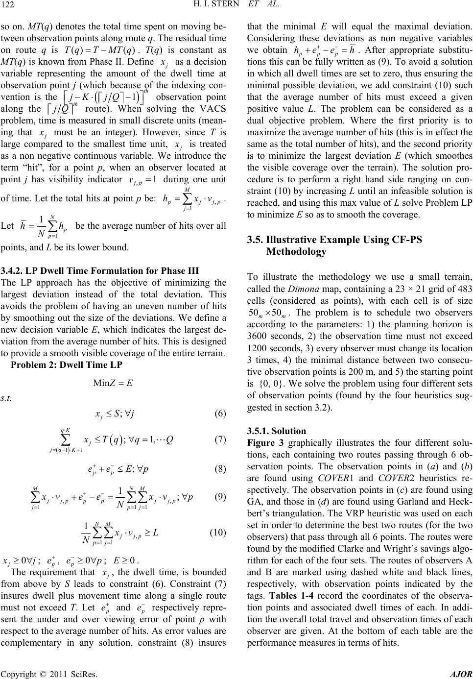

122 H. I. STERN ET AL.
so on. MT(q) denotes the total time spent on moving be-
tween observation points along route q. The residual time
on route q is ()()TqT MTq . T(q) is constant as
MT(q) is knownfine from Phase II. De
j
x
as a decision
variable representing the amount of thdwell time at
observation point j (which because of the indexing con-
vention is the
e

1th jK jQ

 



observation point
along the th


route). When s
is me
jQ

olving the VACS
problem, timasured in small discrete units (mean-
ing that
e
j
x
must be an integer). However, since T is
large comred to the smallest time unit, pa
j
x
is treated
as a non negative continuous variable. We roduce the
term “hit”, for a point p, when an observer located at
point j has visibility indicator ,1
jp
v during one unit
of time. Let the total hits at point
M
int
p be: ,
1
p
jjp
j
hxv
.
Let
1
1
N
p
p
hh
N

points, and L
.4.2. LP DweI
g the
be the average num
be its lower bound.
ll Time Formulation for
ber of
Ph
hits over all
3ase II
The LP approach has the objective of minimizin
largest deviation instead of the total deviation. This
avoids the problem of having an uneven number of hits
by smoothing out the size of the deviations. We define a
new decision variable E, which indicates the largest de-
viation from the average number of hits. This is designed
to provide a smooth visible coverage of the entire terrain.
Problem 2: Dwell Time LP
Min
Z
E

;
j
s.t.
x
Sj


11
;1
qK
j
jq K
,
(6)
x
Tq q




;
pp
eeEp


Q (7)
(8)
,
1
,
1
;
j p
pj 1
1M
jjp pp
j
MN
j
x
vee
N

 
 xv


p (9)

,jj p
11
1NM
pj
x
vL
N


 (10)
0
j
x
j;
p
e,
irem
0
p
ep
;
ent that
0. E
The requ
j
x
, the dwell time, is bounded
from above by S leads tonstraint (6). Constraint (7)
insures dwell plus movement time along a single route
must not exceed T. Let
o c
p
e and
p
e respectively repre-
sent the under and over viewing ror of point p with
respect to the average number of hits. As error values are
complementary in any solution, constraint (8) insures
that the minimal E will equal the maximal deviation.
Considering these deviations as non negative variables
we obtain
er
ppp
hee h


. After appropriate substitu-
tions this caen as (9). To avoid a solution
in which all dwell times are set to zero, thus ensuring the
minimal possible deviation, we add constraint (10) such
that the average number of hits must exceed a given
positive value L. The problem can be considered as a
dual objective problem. Where the first priority is to
maximize the average number of hits (this is in effect the
same as the total number of hits), and the second priority
is to minimize the largest deviation E (which smoothes
the visible coverage over the terrain). The solution pro-
cedure is to perform a right hand side ranging on con-
straint (10) by increasing L until an infeasible solution is
reached, and using this max value of L solve Problem LP
to minimize E so as to smooth the coverage.
n be fully writt
.5. Illustrative Example Using CF-PS
o illustrate the methodology we use a small terrain,
3Methodology
T
called the Dimona map, containing a 23 × 21 grid of 483
cells (considered as points), with each cell is of size
50 50
mm

. The problem is to schedule two observers
to the parameters: 1) the planning horizon is
3600 seconds, 2) the observation time must not exceed
1200 seconds, 3) every observer must change its location
3 times, 4) the minimal distance between two consecu-
tive observation points is 200 m, and 5) the starting point
is {0, 0}. We solve the problem using four different sets
of observation points (found by the four heuristics sug-
gested in section 3.2).
according
3.5.1. Solution
ically illustrates the four different solu-Figure 3 graph
tions, each containing two routes passing through 6 ob-
servation points. The observation points in (a) and (b)
are found using COVER1 and COVER2 heuristics re-
spectively. The observation points in (c) are found using
GA, and those in (d) are found using Garland and Heck-
bert’s triangulation. The VRP heuristic was used on each
set in order to determine the best two routes (for the two
observers) that pass through all 6 points. The routes were
found by the modified Clarke and Wright’s savings algo-
rithm for each of the four sets. The routes of observers A
and B are marked using dashed white and black lines,
respectively, with observation points indicated by the
tags. Tables 1-4 record the coordinates of the observa-
tion points and associated dwell times of each. In addi-
tion the overall total travel and observation times of each
observer are given. At the bottom of each table are the
performance measures in terms of hits.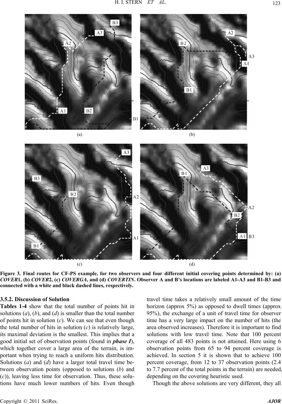

H. I. STERN ET AL.
123
(a) (b)
(c) (d)
Figure 3. Final routes for CF-PS covering points determined by: (a)
.5.2. Discussi on of Solution
l number of points hit in
travel time takes a relatively small amount of the time
example, for two observers and four different initial
COVER1, (b) COVER2, (c) COVERGA, and (d) COVERTIN. Observer A and B’s locations are labeled A1-A3 and B1-B3 and
connected with a white and black dashed lines, respectively.
3
Tables 1-4 show that the tota
solutions (a), (b), and (d) is smaller than the total number
of points hit in solution (c). We can see that even though
the total number of hits in solution (c) is relatively large,
its maximal deviation is the smallest. This implies that a
good initial set of observation points (found in phase I),
which together cover a large area of the terrain, is im-
portant when trying to reach a uniform hits distribution.
Solutions (a) and (d) have a larger total travel time be-
tween observation points (opposed to solutions (b) and
(c)), leaving less time for observation. Thus, these solu-
tions have much lower numbers of hits. Even though
horizon (approx 5%) as opposed to dwell times (approx
95%), the exchange of a unit of travel time for observer
time has a very large impact on the number of hits (the
area observed increases). Therefore it is important to find
solutions with low travel time. Note that 100 percent
coverage of all 483 points is not attained. Here using 6
observation points from 65 to 94 percent coverage is
achieved. In section 5 it is shown that to achieve 100
percent coverage, from 12 to 37 observation points (2.4
to 7.7 percent of the total points in the terrain) are needed,
depending on the covering heuristic used.
Though the above solutions are very different, they all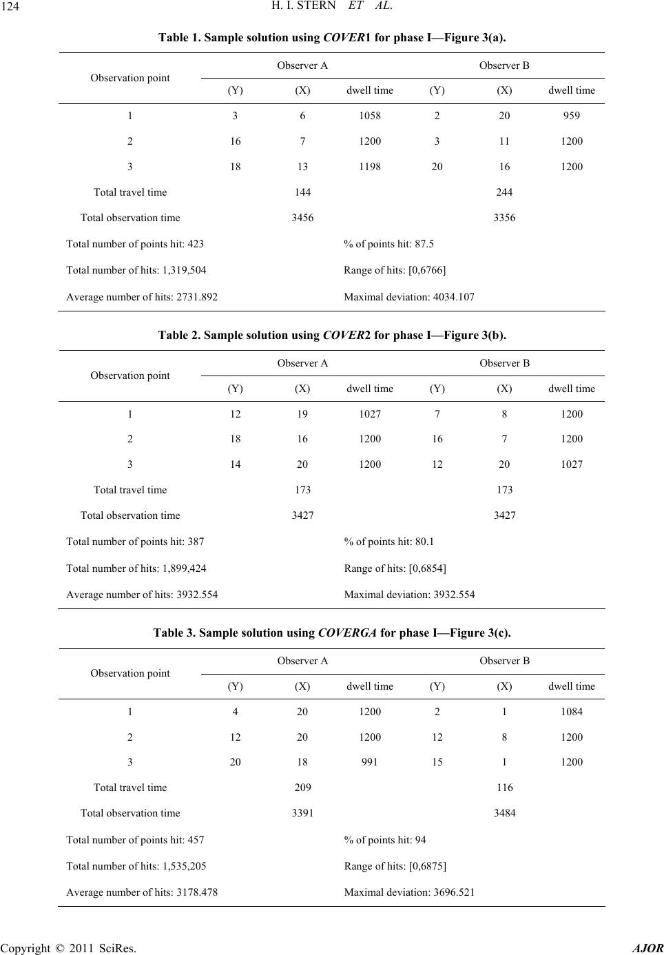

H. I. STERN ET AL.
124
solution using COVE
r B
Table 1. SampleR1 for phase I—Figure 3(a).
Observer A Observe
Observation point
(Y) dwell time (Y) dwell time (X) (X)
1 3 6 1058 2 20 959
2 16 7 1200 3 11 1200
3 18 13 1198 20 16 1200
Total trl time
Toe
To423 % of points hit: 87.5
]
2 107
ave144 244
tal observation tim3456 3356
tal number of points hit:
Total number of hits: 1,319,504 Range of hits: [0,6766
Average number of hits: 2731.89Maximal deviation: 4034.
Table 2. Sample solution using COVER2 for phase I—Figure 3(b).
r B Observer A Observe
Observation point
(Y) (X)
dwell time(Y) (X) dwell time
1 12 19 1027 7 8 1200
2 18 16 1200 16 7 1200
3 14 20 1200 12 20 1027
Total trl time
Toe
To387 % of points hit: 80.1
]
4 554
ave173 173
tal observation tim3427 3427
tal number of points hit:
Total number of hits: 1,899,424 Range of hits: [0,6854
Average number of hits: 3932.55Maximal deviation: 3932.
Table 3. Sample solution using COVERGA for phase I—Figure 3(c).
r B Observer A Observe
Observation point
(Y) (X) dwell time(Y) (X) dwell time
1 4 20 1200 2 1 1084
2 12 20 1200 12 8 1200
3 20 18 991 15 1 1200
Total trl time
Toe
To457 % of points hit: 94
75]
8 521
ave209 116
tal observation tim3391 3484
tal number of points hit:
Total number of hits: 1,535,205 Range of hits: [0,68
Average number of hits: 3178.47Maximal deviation: 3696.

H. I. STERN ET AL.
125
le solution using COV e 3(d).
B
Table 4. SampERTIN for phase I – Figur
Observer A Observer
Observation point
(Y) dwell time(Y) dwell time (X) (X)
1 4 18 1200 16 7 1200
2 10 20 1016 8 17 1004
3 17 11 1200 4 20 1200
Total trl time
Toe
To315 % of points hit: 65.2
]
2 387
ave184 196
tal observation tim3416 3404
tal number of points hit:
Total number of hits: 1,091,393 Range of hits: [0,6811
Average number of hits: 2259.61Maximal deviation: 4551.
ow a reper focuses on a
.1
y contains three phases, starting with a
presentation of the
sh
d
eating pattern. Each observ
ifferent part of the area. This strengthens the idea that
another methodology can be applied here as well. This
method would first divide the area between the observers
(such that each one will have its own region), and then
create a route for each observer within its own region.
This method starts with partitioning and then finds a
covering route for each region, and therefore, it is classi-
fied as “partition first, cover second”. This solution
methodology is discussed in the next section.
4. The Partition First, Cover Second
(PF-CS) Heuristic
. Overview 4
This methodolog
terrain triangulation of a given resolution, partitioning it
into Q regions, one for each observer. In phase I area
partitioning is done starting with a triangle irregular
networks (TINs), where the basic primitives are the tri-
angles. Initial creation of this triangulation is done using
Garland and Heckbert’s Algorithm [14] and is based on a
desired resolution level. We create a partitioning of the
area into Q sub areas (comprised of contiguous triangles),
one for each observer. In a second phase, K points in
each region are found which provide the maximum visi-
ble cover and then a route for every region is created.
The observation times at each point on the routes are
determined using a LP in the third phase. Once there are
Q routes, we solve LP dwell time problem to find the
dwell times for each observer at each observation point.
Figure 4 provides a flowchart of the methodology.
4.2. Phase I—Area Partitioning
Partitioning starts with a given TIN re
Figure 4. Flow chart of the PF-CS methodology.
terrain, with n triangle primitives, denoted as . Trian-
gles are combined to form a “Q-partition”. A Qartition
T ih
T
-p
of
th
s comprised of Q subsets 1,,,,
iQ
TTT of T suc
at; i
TT

 and ij
TT


 ,ij. The area partition
problem is to find a T-partition of T such that the areas of
subsets i
T are close to equal. In addition, all the trian-
gles in T are contiguous, such triangles
share a common side. A Q-partition may be obtained
through an iterative process, starting with n triangles and
joining ctiguous triangles until there are Q continuous,
non-empty regions such that each region contains a finite
number of triangles from the original TIN. To cover a
region containing n vertices, at most

i
on
that any two
12n

of its
vertices are used. Figure 5(a) shows a narrow region
containing 18 triangles. Note, that only the vertices 2, 4,
6 and 8 are needed to cover this region. Figure 5(b)

126 H. I. STERN ET AL.
(a)
(b)
Figure 5. (a) A narrow region; (b) The use of vertices as
observation points.
shows a 3D TIN representation of a small map contain-
ons with the same area are allowed
5], and therefore a heuristic is needed. However, for
he balanced area partition problem can be formulated as
g binary
variab ed
to 0 ot
ing 70 vertices. The partition problem is NP-Hard even
when only two regi
[1
small problems a binary integer formulation is proposed.
4.2.1. Binary Integer Linear Programming
Formulation of the Balanced Area Partition
(BAP) Problem
T
a 0-1 integer programming problem by definin
les ,1
ij
x if triangle

1, ,jj n is assign

1, ,i Q, and
i
Therwise. Let
j
a represent
the area of triangle j, i
A
the area of i T, such that
,ijij
j
A
ax; i and A the area of T. Let


,TAij
be ency indicator, equal to 1 triangles i
and j are adjacent, an0 otherwise. he following is
a triangle adjacif
d Ta
formulation fmi E from
the balanced area state
or nimizing the largest deviation
A
Q
,
1
;
ji j ii
j
axeeAQ i


n


 (11)
;
ii
eeE
 i


(12)
,

,
1
,;,
n
ij ik
k
x
TAj kxij


 (13)
,1;
Q
ij
i
x
j
 (14)


,0,1 , ij
x
ij; ,
ii
ee i


; 0E.
Note that ei

, i
e

are the deviation errors which can
be shown to limentary. Constraint
the target area whe actual area
ment . Co12) states that the deviation error is
E. Cstrain13) states that if a
tri
in
angles attached to
at vertex, and iteratively adds vertices to that region
this
occurhe region growing
be
nstra
a
ssig
comp
ith t
int (
x error
ed
(11) compares
of each partition ele-
i
T
below the m
ai
ont (
angle j is an to i T then it must be adjacent to at
least one of the other triangles assigned to i T. This in-
sures that the set of triangles in any i
T are contagious.
Constrnt (14) insures that each triangle j is assigned to
exactly one triangular subset i T. Note that the problem
does not consider the “compactness” of the triangular
subsets, and thus long narrow subsets may be obtained.
Because integer nonlinear programmg problems re-
quire long solution times we propose the following fast
heuristic to determine the Q-partition.
4.2.2. A Greedy Algorithm for the Balanced Area
Partitioning (BAP) Problem
The greedy area partitioning heuristic starts with a single
vertex, creates a region from all the tri
th
until either of two conditions is violated. When
s a new region is established. T
stopping conditions are: 1) the area of the region must
not exceed the area of the terrain divided by the number
of observers (balanced area), and 2) the distance between
the two furthest points within each region must not
exceed a predefined distance (this avoids long narrow
regions). The triangulation T is represented as a graph
{,}GV

 where, V is the set of vertices, and

is the
set of arcs. Let NA be a node adjacency matrix nn

matrix with common element ,1
ij

 if vertices i and j
are adjacent (both vertices appear in the same triangle),
and 0 otherwise. Let ti V represent a set of all triangles
o vertex i. Let

i
connected t
A
V represent the al area
of the triangles attached to vertex i. The BAP algor
can be shown to be polynomialr

2
On .
The BAP algorithm
1) Calculate
tot
ithm
of orde


i
A
Vor every vertex iV. Sort the
vertices in descending order

i
of the Q-partition.
Problem 3: Balanced area partition integer program
Min
Z
E

s.t.
f
of
A
V. Let 1j

and
let c be the first vertex in the list.
2) Add vertex c to region
j
T. a) Delete vertex c from

H. I. STERN ET AL.
127
th rtex iV

, if tc ti VV



V
e list. b) For every ve, de-
cron triease the commangle's areas out of Ai such that;
 
iititc
A
VAVAVV, i

.
ng
c)
o
Solist o
rder according to
rt the f the
remaining vertices V in decreasi

i
A
V. d) Find the next verte in V which is a neighbor
of one of the vertices in the current regi
x c
on
j
T, and
tex
adds
the largest area to the region, i.e. find a verc such that,


,k j
v.
3) If at least one of the above mentioned two condi-
s violated, then a new region is established. Let
1jj
. Find c, among unassigned vertices, with the
max area:

arg
tions i
1
iik
cMaxAV T  

argcMaxAVvV. Go to step 2.
ii
V
4) Repeat steps 2 and 3 until


n of the region proviQ
, a
.
In
4.3. Phase II—Finding Covering Routes
The partitio smaller probledes
Kms. each we need to locate onlynd not
M
QK


sec-obser
m
resent
vation points using the
instead of the Q vehicleg
Methodology
ate the methodology we
ed in Figure 3 and the
COVER
routin
e sam
Table 5.
1
ob-
p the
a
terrain
of the
uristic
fter performing the partitioning into two regions we get
shown in Figure 6(a). Observer A is
he terrain was divided into the two regions presented in
er A to the north-western
A samthe
Observer B
heuristic (see
ing pr
roblem as in
ints with
use the same
assumptions
P he
ple solution using
tion 3.2.1), and then solve a single vehicle rout
le
previous approach. The routing problem becomes one of
a simple shortest path problem through K po
given start point and an open end point.
4.4. Phase III—Assigning Dwell Times
After creating the routes, the LP dwell time problem is
solved.
over a triangulation with a 5 m level of accuracy. In
phase II the COVER1 heuristic is used in each region to
find the location of the 3 observation points, followed by
the use of the modified savings algorithm to find the
route through each set of points in each region. Phase III
uses the dwell time LP in order to determine the observa-
tion time at each observation point.
4.5.1. Solution
Observer A
A
the two regions
assigned to the area colored gray and observer B is as-
signed to the area colored white. To help the reader visu-
alize the triangulation, a picture of the terrain from the
same view point is given in Figure 6(b). The covering
points found and the two routes through them are shown
in Figures 6(c) and (d). The labels in the figures show
the covering points, and the routes of observers A and B
are indicated by the dashed white and black lines, re-
spectively. Table 5 shows the coordinates of the obser-
vation points and their associated dwell times. In addi-
tion the total travel and observation times of each ob-
server are given. At the bottom of each table are the per-
formance measures in terms of hits.
4.5.2. Discussi on of Solution
T
Figure 6(a), assigning observ
region, and observer B to the eastern region. Table 5
shows that the total number of points hit in this solution
(and therefore the % of area covered) is better than in
solutions 6(a), (b), and (d) for the previous CF-PS exam-
ple, but yet its maximal deviation is larger. One can see
that the dwell LP worked as it did seem to push down the
deviation above the mean 6859 – 4075 = 2784. The max
dev of 4075 is the same as the mean, meaning it occurred
area partitioning methodology.
4.5. Illustrative Example Using PF-CS
To illustr
p
CF-PS example. Phase I uses the greedy BA
Observation point
(Y) (X) dwell time (Y) (X) dwell time
1 10 13 1200 8 1200 1
2
Total trl time134
Total obsetion ti3393 3466
Total 36 % of points hit: 90.2
To430 Range of hits: [0,6859]
4 75.424
13 20 1200 15 1 1066
3 4 20 993 16 8 1200
ave
me
it: 4
,
207
rva
number of points h
tal number of hits: 1,968
Average number of hits: 4075.42Maximal deviation: 40

128 H. I. STERN ET AL.
(a) (b)
(c) (d)
Figure 6. Partitioning of the map into two regions, anesultant routes for PF-CS example. (a) TIN represetation of the
terrain and its partition into two regions; (b) anotheof the partition; (c) final routes and observation pints; (d) 3D
visualization of the solution.
high (each point was seen
075 times or seconds on average) which is good, as it
everal tests were conducted to compare the quality of
r the VACS problem using both
F-PS and PF-CS decomposition heuristics. The tests
were tested; 1) Dimona map, grid = 23 × 21, terrain area
= 1 × 1 km, 2) Modiin map, grid = 61 × 61, terrain area =
d the rn
r view o
between 0 hits (points not seen) and the mean 4075. This
is because the mean was very
of maps, differing by size and topographic structures,
4
implies the total number of hits was also very high.
5. Performance Comparison of CF-PS and
PF-CS Decomposition Methods
5.1. Test Parameters
S
the solutions achieved fo
C
examined the solutions found by the methodologies for
three maps and two scenarios, using 4 and 3 different
versions of the CF-PS and PF-CS methods, respectively.
This resulted in a total of 42 test cases. The performance
of both methodologies was evaluated by function (1),
which represented the total visibility of the terrain by all
observers, penalized for multiple coverage. Three types
3 × 3 km, 3) Valley of Elah map, grid = 81 × 82, terrain
area = 4 × 4 km. Figure 7 shows the terrains, where con-
tour lines are 10 meters apart. The various grid sizes rep-
resent up to a 400 Percent scale up of the problem size.
For the CF-PS method the original rectangular grid point
height representation of the terrain is used. Four covering
versions are tested (COVER1, COVER2, COVERGA and
COVERTIN) for this method. For the PF-CS method the
grid height maps are converted to TIN representations.
Three different TIN versions are tested, each represent-
ing different approximations of the terrain. These are
denoted as TIN5, TIN10 and TIN20 for approximations
of 5 m, 10 m, and 20 m levels of accuracy.
Observation missions can have different objectives
according to different scenarios. This can have a large
effect on the desirable number of relocations and the
allowable observation dwell times. We chose to examine
the two following scenarios:

H. I. STERN ET AL.
129
(a) (b) (c)
Figure 7. 3D contour maps of the three tested terrains.
First scenario:
territory to locate an object (such
he observers must visibly cover t
p
tly a different partitioning dif-
re obtained. The performance value
-
observer and their obser-
) represents the solution
ined by solving problem LP. The
VA and the LP was solved
Observation teams are sent to enemy 5.2. Test Results
as a crashed aircraft).
he entire terrain while Table 7 presents the test results using CF-PS and PF-CST
s ending limited time at any location. Every point must
be viewed just enough to determine if the object exists.
An observer must move so the distance between loca-
tions exceeds a minimum distance to avoid detection.
This type of scenario dictates the use of many observa-
tion points (for complete coverage) without spending too
much time in each. Thus, the maximal dwell time S at
every observation point is relatively small.
Second scenario: Several observation teams are in
enemy territory looking for rocket launchers. Rockets
can be launched from almost any point within the terrain
at any time. Since rocket locations are unknown, it is
desirable for observers to use large coverage points for
quick detection of launchers. Here also the team’s moves
must exceed a minimum distance. This type of scenario
dictates the use of fewer observation points spending a
relatively large time at each, such that large areas will be
visible. The maximal dwell time S should be relatively
large.
Table 6 presents the values for; Q- the number of ob-
servers for each map, K- the number of observation
points for each route, S- the maximal allowed observa-
tion dwell time in seconds at each observation point, d-
the minimal distance between every two consecutive
points, and T- the planning horizon. Note that more ob-
servation points were used for the larger sized terrains
and for the first scenario.
In addition, a sensitivity analysis was made (using the
CF-PS method, and the Dimona map) to study the affect
of the number of observation points on the percent of
area (terrain points) covered. Finally, all of results were
subjectively evaluated by soliciting the opinion of sev-
eral experts in the field.
methodologies (values = 1st scenario/2nd scenario). Since
the 3 versions of the PF-CS correspond to three TIN ap-
proximations with a different number of triangles and
uenvertices, and conseq
rent solutions wefe
was calculated using the objective of the VACS problem
(Equation (1)). This function sums the total number of
viewable points within the terrain to all observers (not
including overlaps) throughout the entire planning hori-
zon, giving an exponentially decreasing contribution
(starting from 1 and going to 0) to each visible point ac-
cording to the number of times it was previously seen.
5.3. Two Sample Solutions
Figure 8 illustrates the solution using both methodolo-
gies for a 16 km2 terrain of the Valley of Elah (the area in
which David confronted Goliath). There are three observ-
rs, each changing its location 3 times. The labels indie
cate the order of visits of each
ation time (sec.). Figure 8(a v
achieved by the CF-PS methodology using COVERGA
for phase I. Figure 8(b) represents the solution achieved
by the PF-CS methodology based on a TIN with a 5 m
level of accuracy.
5.3.1. CF-PS (Figure 8(a))
The set of covering points was selected using GA (Phase
I) which was found to give good visual coverage. In
Phase II the routes where generated using the modified
savings algorithm In Phase III the observation dwell
mes where determti
code was implemented in JA

H. I. STERN ET AL.
130
Table 6. Test parameters for all maps and scenarios (table values are 1st scenario/2nd scenario).
Map Q K S d T
Dimona 2/2 5/3 600/1200 200/200 3600/3600
M60000 4000 72000
Va h
odiin 3/2 5/4 /180/4 0/72
lley of Ela3/3 8/3 600/2400 500/500 7200/7200
F-PS and PF-CS (col 4 and 5 values are for 1st nd scenario)
Performance Value* 104 No. observers, No. points Version Method Map
Table 7. Results for C scenario/2.
21.6/51 2.10/2.6 COVER1
19.1/50.6 2.10/2.6 COVER2
24.5/61.6
2.10/2.6 COVERGA
C
PF-CS
Dimona
1 COVER1
2 COVER2
COVERGA
C
CF-PS
PF-CS
Modiin
COVER1
COVER2
COVERGA
C
CF-PS
PF-CS
Valley of Elah
14.3/29.4 2.10/2.6 OVERTIN
CF-PS
23.4/60.5 2.10/2.6 TIN 20
23.5/62.8 2.10/2.6 TIN 10
23.8/62.9
2.10/2.6 TIN 5
97.7/484.23.15/2.8
36.9/527.33.15/2.8
292.7/716.5 3.15/2.8
186.6/358.2 3.15/2.8 OVERTIN
275/645.5 3.15/2.8 TIN 20
290/673.4 3.15/2.8 TIN 10
285.6/642.9 3.15/2.8 TIN 5
409.6/1426 3.24/3.9
423.5/1451 3.24/3.9
569.6/2024 3.24/3.9
507.3/1810 3.24/3.9 OVERTIN
555.9/1896 3.24/3.9 TIN 20
566.3/1946 3.24/3.9 TIN 10
566.2/1946
3.24/3.9 TIN 5
using Matlab. This solution pr a clear area
tioning between the observers. Observer C moves along
e western ridge (advancing from south to north), which
5.3.2. PF-(Figure 8(b))
In Pha area was partthe three regions
for a terrain triangulation of 5 m accuracy. In Phase II
h observer focuses on a re-
s sent to the north-western
oduces parti-
th
visually covers the entire valley and most of the gorges
which flow from east to west. Observer B covers the
southern part of the terrain moving from west to east.
Observer A covers the northern side of the terrain with
its deep gorges, which are not visible from the western/
southern ridge.
the observation points in each region were selected using
a greedy SCP heuristic, and the routes which pass through
them were generated using the shortest path algorithm.
Phase III also used the LP problem. In this solution we
CS
se I theitioned to
can see once again that eac
stricted region. Observer A i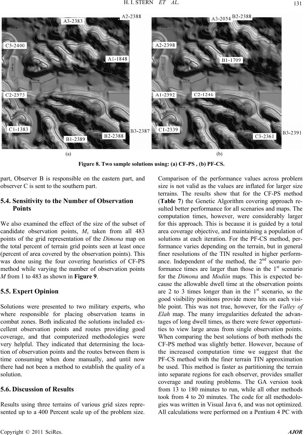

H. I. STERN ET AL.
131
(a) (b)
Figure 8. Two sample solutions using: (a) CF-PS , (b) PF-CS.
part, Observer B is responsible on the eastern part, and
observer C is sent to the s
.4. Sensitivity to the Num
of the subset of
83
on
e tof terrain grid points seen at least once
n teams in
cated the solutions included ex-
nts and routes providing good
o a 400 Percent scale up of the problem size.
Comparison of the performance values across problem
es are inflated for larger size
that for the CF-PS method
rithm covering approach re-
ulted better performance for all scenarios and maps. The
were considerably larger
guided by a total
outhern part. size is not valid as the valu
5ber of Observation terrains. The results show (Table 7) the Genetic Algo
Points
e also examined the effect of the size W
candidate observation points, M, taken from all 4
points of the grid representation of the Dimona map
otal percent th
(percent of area covered by the observation points). This
was done using the four covering heuristics of CF-PS
method while varying the number of observation points
M from 1 to 483 as shown in Figure 9.
5.5. Expert Opinion
Solutions were presented to two military experts, who
here responsible for placing observatiow
combat zones. Both indi
ellent observation poic
coverage, and that computerized methodologies were
very helpful. They indicated that determining the loca-
tion of observation points and the routes between them is
time consuming when done manually, and until now
there had not been a method to establish the quality of a
solution.
5.6. Discussion of Results
Results using three terrains of various grid sizes repre-
sented up t
s
computation times, however,
r this approach. This is because it is fo
area coverage objective, and maintaining a population of
solutions at each iteration. For the PF-CS method, per-
formance varies depending on the terrain, but in general
finer resolutions of the TIN resulted in higher perform-
ance. Independent of the method, the 2nd scenario per-
formance times are larger than those in the 1st scenario
for the Dimona and Modiin maps. This is expected be-
cause the allowable dwell time at the observation points
are 2 to 3 times longer than in the 1st scenario, so the
good visibility positions provide more hits on each visi-
ble point. This was not true, however, for the Valley of
Elah map. The many irregularities defeated the advan-
tages of long dwell times, as there were fewer opportuni-
ties to view large areas from single observation points.
When comparing the best solutions of both methods the
CF-PS method was slightly better. However, because of
the increased computation time we suggest that the
PF-CS method with the finer terrain TIN approximation
be used. This method is faster as partitioning the terrain
into separate regions for each observer, provides smaller
coverage and routing problems. The GA version took
from 13 to 180 minutes to run, while all other methods
took from 4 to 20 minutes. The code for all methodolo-
gies was written in Visual Java 6, and was not optimized.
All calculations were performed on a Pentium 4 PC with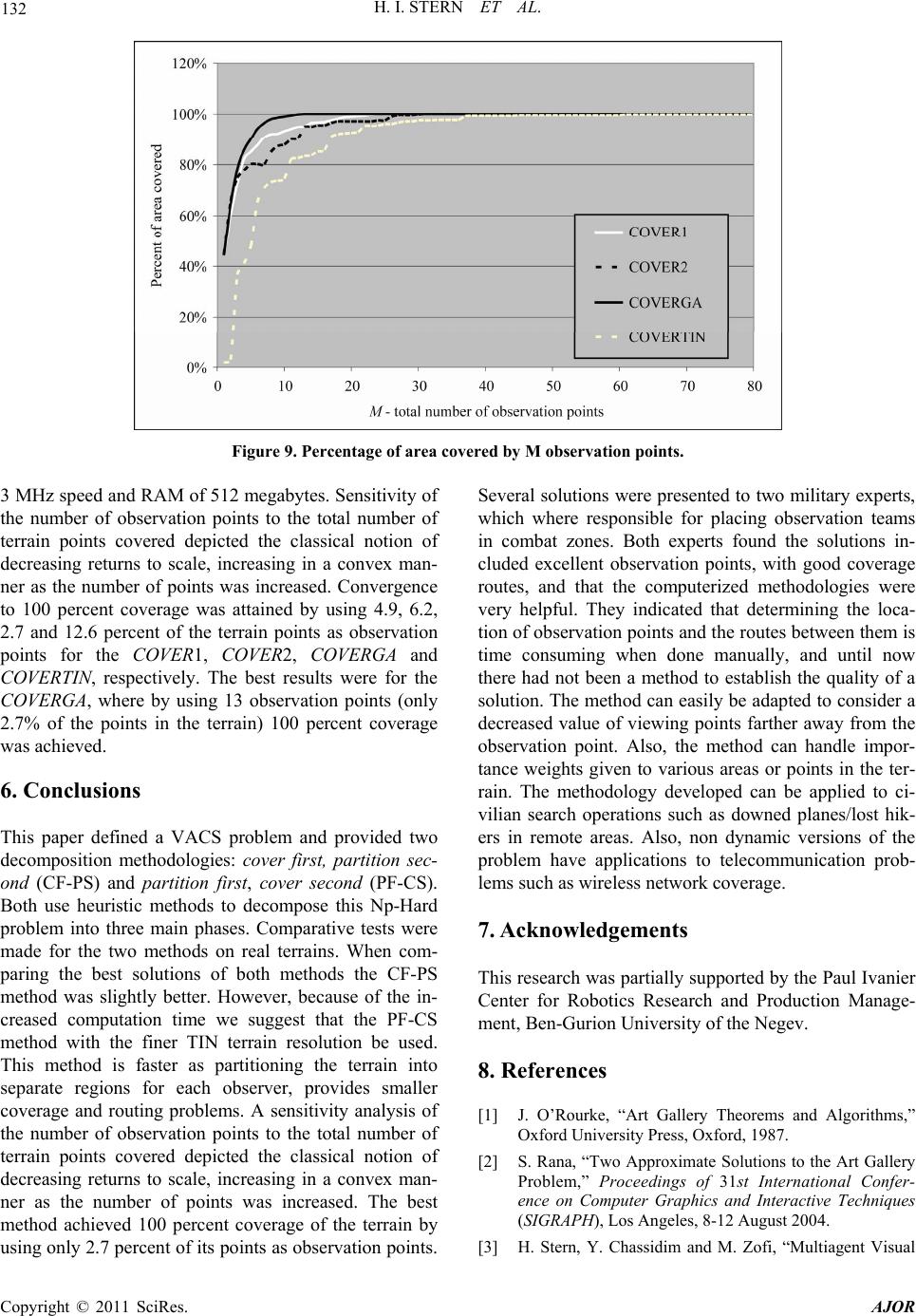

132 H. I. STERN ET AL.
Figure 9. Percentage of area covered by M observation points.
3 MHz speed and RAM of 512 megabytes. Sensitivity of
the number of observation points to the total number of
terrain points covered depicted the classical notion of
decreasing returns to scale, increasing in a convex man-
ner as the number of points w
100 percent coverage was attained by using 4.9, 6.2,
d partition first, cover second (PF-CS).
ethods to decompose this Np-Hard
ain phases. Comparative tests were
ade for the two methods on real terrains. When com-
Several solutions were presented to two military experts,
which where responsible for placing observation teams
in combat zones. Both experts found the solutions in-
cluded excellent observation points, with good coverage
terized methodologies were
very helpful. They indicated that determining the loca-
the Art Gallery
Problem,” Proceedings of 31st International Confer-
ics and Interactive Techniques
August 2004.
as increased. Convergence routes, and that the compu
to
2.7 and 12.6 percent of the terrain points as observation
points for the COVER1, COVER2, COVERGA and
COVERTIN, respectively. The best results were for the
COVERGA, where by using 13 observation points (only
2.7% of the points in the terrain) 100 percent coverage
was achieved.
6. Conclusions
This paper defined a VACS problem and provided two
decomposition methodologies: cover first, partition sec-
ond (CF-PS) an
Both use heuristic m
problem into three m
m
paring the best solutions of both methods the CF-PS
method was slightly better. However, because of the in-
creased computation time we suggest that the PF-CS
method with the finer TIN terrain resolution be used.
This method is faster as partitioning the terrain into
separate regions for each observer, provides smaller
coverage and routing problems. A sensitivity analysis of
the number of observation points to the total number of
terrain points covered depicted the classical notion of
decreasing returns to scale, increasing in a convex man-
ner as the number of points was increased. The best
method achieved 100 percent coverage of the terrain by
using only 2.7 percent of its points as observation points.
tion of observation points and the routes between them is
time consuming when done manually, and until now
there had not been a method to establish the quality of a
solution. The method can easily be adapted to consider a
decreased value of viewing points farther away from the
observation point. Also, the method can handle impor-
tance weights given to various areas or points in the ter-
rain. The methodology developed can be applied to ci-
vilian search operations such as downed planes/lost hik-
ers in remote areas. Also, non dynamic versions of the
problem have applications to telecommunication prob-
lems such as wireless network coverage.
7. Acknowledgements
This research was partially supported by the Paul Ivanier
Center for Robotics Research and Production Manage-
ment, Ben-Gurion University of the Negev.
8. References
[1] J. O’Rourke, “Art Gallery Theorems and Algorithms,”
Oxford University Press, Oxford, 1987.
[2] S. Rana, “Two Approximate Solutions to
ence on Computer Graph
(SIGRAPH), Los Angeles, 8-12
[3] H. Stern, Y. Chassidim and M. Zofi, “Multiagent Visual

H. I. STERN ET AL.
133
jor.2005.02.078
Area Coverage Using a New Genetic Algorithm Selection
Scheme,” European Journal of Operational Research
Vol. 175, No. 3, 2006, pp. 1890-1907.
,
doi:10.1016/j.e
hassidim, M. Zofi and M. Kaspi, “Multi
elligence and
on, Sarasota
. 2, 1981, pp. 186-197.
[4] H. Stern, Y. C
Agent Visual Area Coverage Strategies Using an Adap-
tive Queen Genetic Algorithm,” Proceedings of IASTED
International Conference on Artificial Int
Applications, Innsbruck, 14-16 February 2005.
[5] W. R. Franklyn, “Applications of Analytical Cartogra-
phy,” Handbook of Discrete and Combinatorial Mathe-
matics, CRC Press, Boca Raton, 2000.
[6] M. Marengoni, B. A. Draper, A. Hanson and R. Sitara-
man, “Placing Observers to Cover a Polyhedral Terrain in
Polynomial Time,” Proceedings of the 3rd IEEE Work-
shop on Applications of Computer Visi
December 1996, pp. 1-6.
, 2-4
[7] V. V. Vazirani, “Approximation Algorithms,” Springer-
Verlag, Berlin, 2001.
[8] M. R. Garey and D. S. Johnson, “Computers and Intrac-
tability: A Guide to the Theory of NP-Completeness,” W.
H. Freeman and Co, San Francisco, 1979.
[9] H. E. Gindy and D. Avis, “A Linear Algorithm for Com-
puting the Visibility Polygon from a Point,” Journal of
Algorithms, Vol. 2, No
doi:10.1016/0196-6774(81)90019-5
[10] D. Cohen-Or and A. Shaked, “Visibility and Dead-Zones
in Digital Terrain Maps,” Computer Graphic s Forum, Vol.
14, No. 3, 1995, pp. 171-180.
doi:10.1111/j.1467-8659.1995.cgf143_0171.x
[11] F. M. Jonsson, “An Optimal Pathfinder for V
Real-World Digital Terrain Maps,” T
ehicles in
he Royal Institute of
hn Wiley
eckbert, “Fast Triangular Ap-
. 113-117.
Science, School of Engineering Physics, Stockholm, 1997.
[12] E. L. Lawler, J. K. Lenstra, A. H. G. R. Kan and D. B.
Shmoys, “The Traveling Salesman Problem,” Jo
& Sons, Hoboken, 1992.
[13] A. Jaszkiewicz, “Comparative Study of Multiple-Objective
Metaheuristics on the Bi-Objective Set Covering Problem
and the Pareto Memetic Algorithm,” Research Report,
Institute of Computing Science, Poznan University of
Technology, Poznań, 2001.
[14] M. Garland and P. S. H
proximation of Terrains and Height Fields,” Proceedings
of SIGGRAPH’97 Conference, Los Angeles, 3-8 August
1997.
[15] B. Hayes, “The Easiest Hard Problem,” American Scien-
tist, Vol. 90, No. 2, 2002, pp
doi:10.1511/2002.2.113
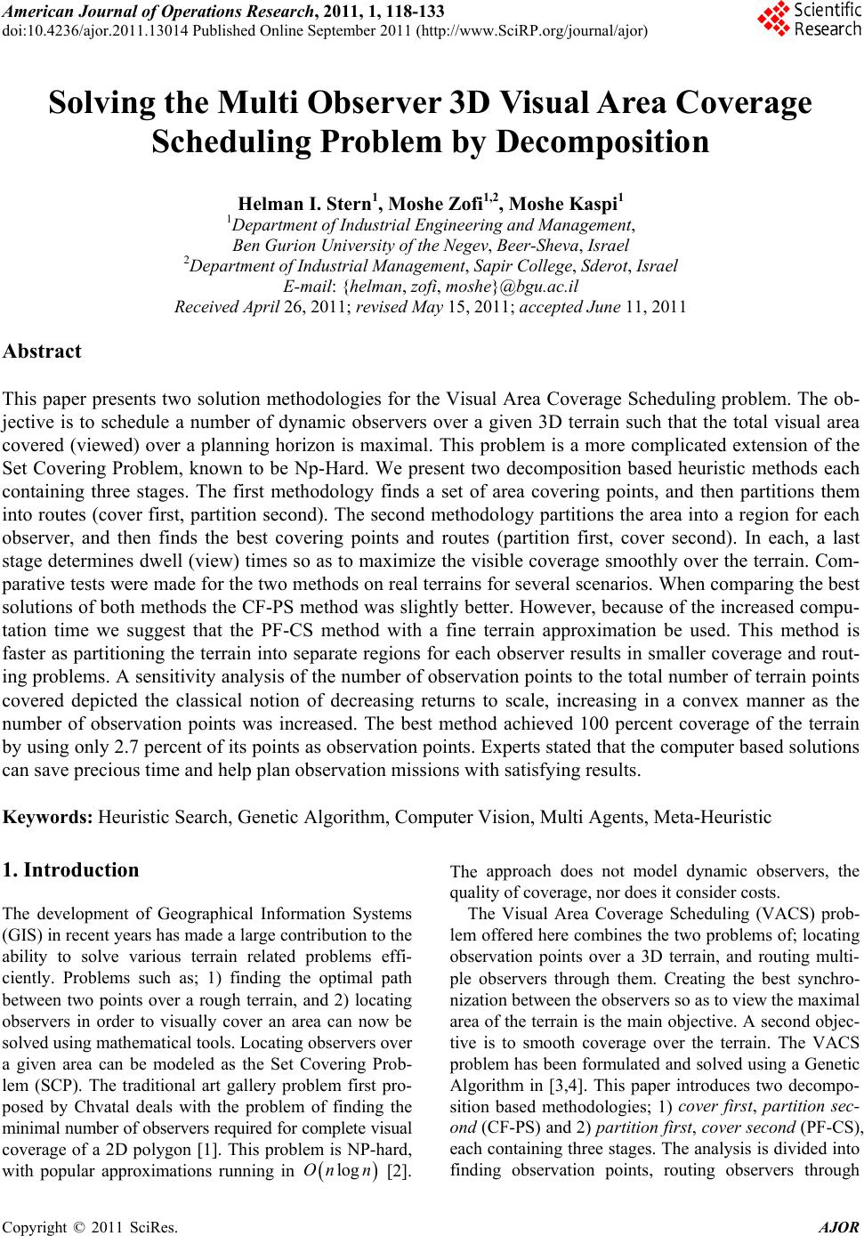