 American Journal of Oper ations Research, 2011, 1, 84-99 doi:10.4236/ajor.2011.13012 Published Online September 2011 (http://www.SciRP.org/journal/ajor) Copyright © 2011 SciRes. AJOR Two-Stage Ordering Policy under Buyer’s Minimum-Commitment Quantity Contract Hsi-Mei Hsu, Zi-Yin Chen Department of Industrial Engineering & Management, National Chaio Tung University, Hsinchu, Chinese Taipei E-mail: hsimei@cc.nctu.edu.tw, yahuilin2@ydu.edu.tw Received July 1, 2011; revised July 22, 2011; accepted August 16, 2011 Abstract In this paper we consider a two-stage ordering problem with a buyer’s minimum commitment quantity con- tract. Under the contract the buyer is required to give a minimum-commitment quantity. Then the manufac- turer has the obligations to supply the minimum-commitment quantity and to provide a shortage compensa- tion policy to the buyer. We formulate a dynamic optimization model to determine the manufacturer’s two stage order quantities for maximizing the expected profit. The conditions for the existence of the optimal so- lution are defined. And we also develop a procedure to solve the problem. Numerical examples are given to illustrate the proposed solution procedure and sensitivity analyses are performed to find managerial insights. Keywords: Two Stages Ordering, Commitment, Bayesian Information Updating 1. Introduction In this paper we study a two-stage component ordering problem with a buyer minimum-commitment quantity contract. Under the contract, the buyer is required to commit a minimum order quantity 1 and for returning the buyer’s commitment the manufacturer has the obli- gations to supply the minimum-commit quantity 1 and to give shortage compensation if the manufacturing sup- ply level is under 1 1 where is a shortage compensation range coefficient 01 . Because of the presence of the long lead time of key components, the manufacturer has two opportunities to place his order to supplier before the buyer’s demand realized. The buyer’s real demand X is uncertain following a normally distribution (0 N ,2 0 ) where 0 is uncertain having a normal distribution N( ,2 1 ). When the manufacturer makes his first order quantity (1) decision at stage 1, the unit cost of key component at stage 1 is known but the unit cost at the stage 2 is uncer- tain. The possible values of and their corresponding probabilities are known, denoted as q (1) c (2) (2) C C (2)(2) (2)(2) 12 ,,, n Ccc c and respe- ctively. After receiving the buyer’s minimum-commit quantity 1 12 ,,, n Ppp p , the manufacturer uses 1 as an estimator of and places his first order quantity (1) to his sup- plier. At stage 2 the marketing department provides an observation 2 q of X. The posterior distribution of X is defined by the observations of 1 and 2 . Then manu- facturer places his second order quantity 2 if necessary. The time events of key component procurement process are shown in Figure 1. q We assume that the outputs are mainly limited by the available amounts of the key component, and the pro- duction cycle times are very short that can be neglected. After receiving the key components, the manufacturer produces the products immediately. Products are deliv- ered to the buyer at the end of period (immediately after second stage). Due to the demand uncertainty, the manu- facturer is difficult to determine two stage order quanti- ties. In this paper we develop a two-stage dynamic optimi- zation model to decide the order quantity of a key com- ponent under a buyer’s minimum-commitment quantity contract. The model is formulated to maximize a manu- facturer’s profit. The following costs are considered in the model. 1) Key component unit cost: the unit cost of key component at stage 1 is and the unit cost at stage 2 is . 2) Holding cost: two kinds of inventories are considered. One is buyer responsible inventory, which only exists in the case of buyer’s real demand (x) below the minimum guaranteed quantity 1 (1) c (2) C . In this case, customers only take away real demand x, and the re- maining products (1 ) are buyer responsible inventory 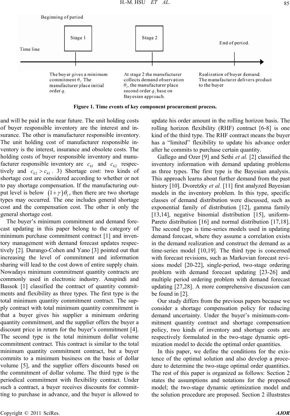 H.-M. HSU ET AL. 85 Figure 1. Time events of key component procurement process. and will be paid in the near future. The unit holding costs of buyer responsible inventory are the interest and in- surance. The other is manufacturer responsible inventory. The unit holding cost of manufacturer responsible in- ventory is the interest, insurance and obsolete costs. The holding costs of buyer responsible inventory and manu- facturer responsible inventory are 1h and 2h c respec- tively and 21hh . 3) Shortage cost: two kinds of shortage cost are considered according to whether or not to pay shortage compensation. If the manufacturing out- put level is below c cc 1 1 , then there are two shortage types may occurred. The one includes general shortage cost and the compensation cost. The other is only the general shortage cost. The buyer’s minimum commitment and demand fore- cast updating in this paper belong to the category of minimum purchase commitment contract [1] and inven- tory management with demand forecast updates respec- tively [2]. Durango-Cohen and Yano [3] pointed out that increasing the level of commitment and information sharing will lead to the cost down of entire supply chain. Nowadays minimum commitment quantity contracts are commonly used in electronic industry. Anupindi and Bassok [1] classified the contract of quantity commit- ments and flexibility as three types. The first type is the total minimum quantity commitment contract. The sup- ply contract with total minimum quantity commitment is that a buyer gives his supplier a minimum ordering quantity commitment, and the supplier offers the buyer a discount price in return for the buyer’s commitment [4]. The second type is the total minimum dollar volume commitment contract. This contract is similar to the total minimum quantity commitment contract, but a buyer commits to a minimum business on the basis of dollar volume [5], and the supplier offers discounts based on the commitment of dollar volume. The third type is the periodical commitment with flexibility contract. Under such a contract, a buyer receives discounts for commit- ting to purchase in advance, and the buyer is allowed to update his order amount in the rolling horizon basis. The rolling horizon flexibility (RHF) contract [6-8] is one kind of the third type. The RHF contract means the buyer has a “limited” flexibility to update his advance order after he commits to purchase certain quantity. Gallego and Ozer [9] and Sethi et al. [2] classified the inventory information with demand updating problems as three types. The first type is the Bayesian analysis. This approach learns about further demand from the past history [10]. Dvoretzky et al. [11] first analyzed Bayesian models in the inventory problem. In this type, specific classes of demand distribution were discussed, such as exponential family of distribution [12], gamma family [13,14], negative binomial distribution [15], uniform- Pareto distribution [16] and normal distribution [17,18]. The second type is time-series models used in updating demand forecast, where they assume a correlation exists in the demand realization and construct the demand as a time-series model [10,19]. The third type is concerned with forecast revisions, such as Markovian forecast revi- sions model [20-22], single-period, two-stage ordering problem with demand forecast updating [23-26] and multiple period ordering problem with demand forecast updating [27,28]. A more comprehensive discussion can be found in [2]. Our study differs from the previous papers because we consider a shortage compensation policy for reducing demand uncertainty. Under the buyer’s minimum-com- mitment quantity contract and shortage compensation policy, two kinds of inventory and shortage costs are respectively formulated in the two-stage dynamic opti- mization model to decide the optimal order quantities. In this paper, we define the conditions for the exis- tence of the optimal solution and also develop a proce- dure to determine the two-stage optimal order quantities. The rest of this paper is organized as follows: Section 2 states the assumptions and notations for the proposed model; the two-stage dynamic optimization model and the solution procedure are proposed. Section 2 illustrates Copyright © 2011 SciRes. AJOR  86 H.-M. HSU ET AL. some numerical examples, and sensitivity analyses of the major parameters of the model are performed. Finally, Section 4 concludes this article. 2. Problem Formulation 2.1. Notations 1 : buyer’s minimum-commitment quantity. 10 : shortage compensation range coefficient 01 . [1 , 1 1 ] is the shortage compensation range. (1 c): unit ordering cost of key component at stage 1. (2) C: unit ordering cost of key component at stage 2 is a random variable, and the corre- sponding probability . (2)(2) (2)(2) 12 ,,, n Ccc c {,, ,} n Ppp p (1) pc 12 : product unit selling price. . p 2 : the demand observation at stage 2. 1h c c: unit holding cost of buyer responsible inventory. 2h: unit holding cost of manufacturer responsible in- ventory. 1 c: unit shortage compensation cost; 10 s c 2 c: unit general shortage cost; 12ss 0cc : buyer’s real demand, realization is denoted by . (1) : (1) is a random variable to forecast the buyer’s demand at stage 1, (1) 1 X . (2) : )(2 is a random variable to forecast the buyer’s demand at stage 2, (2) 12 ,XX . 1(.) : probability density function (pdf) of (1) , 2 2 10 1 ,XN (1) 2(.) : probability density function (pdf) of (2) , (2)22 222 2 12 01010 1 22222 010 01 , XN 1(.) : cumulative density function (cdf) of. (1) 2(.)F: cumulative density function (cdf) of (2) . (.) : standard normal probability density function. (.): the cumulative distribution function for standard normal distribution. 1(.) (.) : inverse function of . (.) : the standard linear loss function: ()()d () a axa x. Decision variables: 1 q q: order quantity at stage 1. 10q 0q 2: order quantity at stage 2. 2 Intermediate variables: 1: the decision space defined by 1 112 (1 )qq (1 )qq . 2 : the decision space defined by 112 . 11 q: optimal order quantity in 1 at stage 1 21 q: optimal order quantity in 1 at stage 2 12 q: optimal order quantity in 2 at stage 1 22 q : optimal order quantity in at stage 2 2 1 q : optimal order quantity at stage 1 2 q : optimal order quantity at stage 2 2.2. Problem Assumptions and Formulation The mathematical model is formulated to determine the two stage ordering quantities of the key component for maximizing profit. The buyer’s real demand X is uncer- tain to be assumed following a normal distribution with an uncertain mean 0 and a given variance 2 0 , where 0 follows N( ,2 1 ) with an unknown and a given variance 2 1 . At stage 1, after receiving the buyer’s minimum commitment quantity 1 , the manufacturer uses 1 as an estimator of . The posterior distribu- tion of X after receiving 1 at stage 1 is denoted as (1) 1 X where (1)2 2 110 ,XXN 1 (1) At stage 2, the marketing department collects informa- tion 2 about buyer’s real demand. We call it as an observation of X. The posterior distribution of X at stage 2 is denoted as (2) 12 ,XX where (2) 2 1222 ,,XX Nk (2) 222222 2 1201 0101 k (3) 222222 201001 (4) Because the manufacturer has the obligation to pro- vide the minimum-commitment quantity 1 to the buyer, the total order quantities 12 must be larger than 1 qq . Now we will formulate the expected profit function and use a backward dynamic programming to determine the optimal 1 q and 2 q . We formulate the problem as a dynamic programming (DP) problem. For the DP formulation, the ordering times are given as the stages, stage 1 and stage 2. Deci- sion variable for stage n (n = 1, 2) is the ordering quan- tity n. The profit at the current stage depends upon the current decision and the ordering quantity in the preceding stage q n q 1n q . We set states for each stage n as 1n q . With the backward solving procedure, first we should determine the optimal order quantity 2 at stage 2 in a given state 2 q 1 q . We denote the expected profit func- tion at stage 2 as (2)2 1 Eqq . The state at stage 1 is known as 10s . The expected profit function at stage 1 is denoted as 1 q (1) E , where (1) (1)11(2)2 1 EqEcqEqq (5) Copyright © 2011 SciRes. AJOR  H.-M. HSU ET AL. Copyright © 2011 SciRes. AJOR 87 The optimal expected profit of the manufacturer is de- termined as follows: lows: 1) Expected products sales 1 1 (1) 1(1) 1 0 (1) 1(2) 21 0 max max q q Eq Eq EcqEqq (6) 122 min, d X p xqqfxx (9) 2) Ordering costs when (2) (2) Cc where (2) 2 cq (10) 2 (2)21(2)21 0 max q Eqq Eqq (7) 3) Expected holding costs: The unit holding cost of buyer responsible inventory is 1h and holding cost of manufacturer responsible in- ventory is . The holding costs can be expressed as follows: c 2h c The items considered in (2)2 1 Eqq are expected product sales, ordering costs, expected holding costs and expected shortage costs. (2)2 1Expected revenues Expected costs Expected product sales Ordering costsExpected holding costs Expected shortage costs Eqq (8) 112 1211 2121 1 for for 0othe hh h cxcqq x cqqx xqq 2 rwise (11) The expected holding costs can be formulated as fol- lows: The relevant items are formulated respectively as fol- 1121212 max,0 max,0d hh X cxcqqxf xx (12) 4) Expected shortage costs: The decision space of total order quantity 21 qq can be divided into two subspaces 1 and , 1 2 : total order quantity (2 ) is less than 1 qq 1 1 2 qq , as shown in Figure 2(a); 2: total order quantity (1) is lar- ger than 1 1 , as shown in Figure 2(b). In 1 , two kinds of shortage types may occur: 1) the shortage oc- curred between and 1 qq2 1 1 belongs to short- age compensation range, its unit shortage costs are the shortage compensation cost and general shortage cost; 2) the others does not belong to shortage compensation range, its unit shortage cost is general shortage cost. The unit shortage costs of shortage compensation and general shortage are 1 c and 2 c respectively, 12 s. In 2 cc , the shortage compensation cost does not occur. Two cases of shortage can be expressed as follows: 112 12 11112 211 for 1, expected shortage costs in 1 + 1for 1, 0ot s ss cxqqqq x cqqcx 1 herwise. x (13) 212 112 2 for 1, expected shortage costs in 0 otherwise. s cxqqqq x (14) Expected shortage cost can be combined as follows: 11122121 maxmin1,,0maxmax, 1,0d ss cxqqcxqq 2 fxx (15) (2)2 1 Eqq depend on the domain of the total order quantity 21 qq , i.e., 112112 1 2.3. Optimal Solution ,1qqqq and ,1q q 11 qq 212 1 To solve the DP problem we first provide the optimal de- cisions for stage 2 under a given state 21 q. As men- tioned above the expected shortage costs in , each domain cor- responds to a shortage cost equation respectively (Figures (a) and (b)). Therefore (2)2 1 Eqq is formulated 2 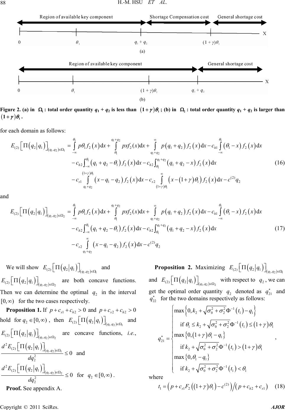 H.-M. HSU ET AL. Copyright © 2011 SciRes. AJOR 88 (a) (b) Figure 2. (a) in : total order quantity q1 + q2 is less than 1 1 1 ; (b) in 2 : total order quantity q1 + q2 is larger than 1 1 . for each domain as follows: 112 1 12 1 112 112 1 1 12 1 (2)211 22122112 , 212122122 1 (2) 1122212 2 1 d()dd dd d1d qq h qq qq qq hh ss qq Eqqpfxxpxfxxpqqfxxc xfx cqqfxxcqqxfxx cxqqfxxcxfxxcq dx (16) and 112 1 12 2 112 112 1 12 (2)211 22122112 , 21212212 2 (2) 2122 2 d()d d dd d qq h qq qq qq hh sqq Eqqpfxxpxfxxpqqfxxcxfx cqqfxxcqqxfxx cxqqfxxcq dx (17) We will show 12 1 (2)2 1,qq Eqq and 12 2 (2)2 1, qq Eqq are both concave functions. Then we can determine the optimal in the interval for the two cases respectively. 2 q [0, ) Proposition 1. If and hold for, then 12 0 sh pc c22 0 sh pc c 2[0, )q 12 1 1, qq q (2)2 Eq and 2 12 (2)2 1, qq Eqq are concave functions, i.e., 12 1 ,0 qq 2 (2)2 1 2 2 dEq q dq and 12 2 2 (2)2 1, 2 2 0 qq dEq q dq for . 2[0, )q Proof. See appendix A. Proposition 2. Maximizing 12 1 (2)2 1,qq Eqq and 12 2 (2)2 1,qq Eqq with respect to , we can 2 q get the optimal order quantity 2 denoted as 21 q q and 22 q for the two domains respectively as follows: 221 202 11 221 12021 11 21 221 202 11 11 221 202 11 max 0, if 1 max0,1 if 1 max0, if ktq kt q q kt q kt 1 , where (2) 1121 2 1 sh tpcFc pcc 1 s (18)  H.-M. HSU ET AL. 89 11 221 12022 22 221 202 21 221 202 21 max0,1 if 1 max 0, if 1 q kt qktq kt 1 , where (2) 22 2 sh tpcc pcc 2 s (19) Proof: See appendix B. Then we provide the optimal solution for stage 1. At stage 1, the profit functions 12 112 1 (1) 11(2)211 (, ), qq qq qcqEqq and 12 212 2 (1) 11(2)221 (, ), qq qq qcqEqq correspond to 1 and 2 respectively. Due to 2 and being uncertain, the sample space of is k )(2) C(2 C (2)) (2(2) 12 , n c ,p (2 Cc 12 {,Pp ) ,,c , } n p with respect to the probability , and the distribution of is 2 k 422 110 1 ,N . Let 12 1 12 1 (1)1 (, ) (1) 1(2) 211 (,) qq qq Eq EcqE qq and 12 2 12 2 (1)1 (, ) (1) 1(2) 221 (, ) qq qq Eq EcqE qq be the expectation of 12 1 1(, ) qq q and 12 2 1(, ) qq q respectively, that are formulated as fol- lows: 1 113 1 2 12 1 12 1 12 12 1 113 1 () (1)1( 2)2122 , (, )1 (1) (2)21221 , () 0, d 0,d nqdd t iK qq qq i K qq qdd t EqpEqqfkk Eqqfkkc q (20) 11 3 2 2 12 2 12 2 12 12 2 113 2 () (1)2 1(2)2122 , (, )1 (1) (2)212 21 , () 0, d 0,d qd d t iK qq qq i K qq qdd t EqpEqq fkk Eqq fkkc 1 n q (21) where 12 1 22 22 (2)211 20 2120 2 , 22 1 21 021 22 22 12021202 22 12112021 (2)2 2 1211202 2 (2) 0, 1 11 11 hh qq hs ss hh s hh s h Eqq pcck pc ct cc k pc cck ccc ckk cc 2222 1 2112020 21 22 (2) 1112021 11 11 , s s ck ckcq t (22) 1 (2) 121 2 11 hs tpcFc pcc Copyright © 2011 SciRes. AJOR  90 H.-M. HSU ET AL. 12 1 22 22 (2)2121021 202 , 22 22 12 021202 22 22 12021202 22 1211202 22 2112021 1 0, 1 11 11 11 hs qq hh ss hh s hs s Eqq pccqk pc ck cc k pc cck cck q c 1 22 1202112 , h kc k (23) 12 2 22 22 (2)211 20 2120 2 , 22 1 22 022121 (2)(2)2 21(2) 1222 0221 (2) 22 22 0, , hh qq hs hh hh h shs Eqq pcck pcctpc c ccckcctcq tpcc pcc (24) 12 2 22 22 (2)212 20 2120 2 , 22 22 12 021202 1211221 0, . hs qq hh hhh h Eqq pccqk pc ck pccckcq (25) Proof: See appendix C. We will show and 12 1 (1)1 ,qq Eq 12 2 (1)1 ,qq Eq are both concave functions. Then we can search for optimal ordering quantity for each domain, expressed as (, 11 q 21 q ) and (, ) respec- tively. 12 q 22 q Proposition 3. If 12 0 sh pcc and 22 0 sh pc c hold for1[0, )q , then and 12 1 (1)1 ,qq Eq 12 1,qq Eq 2 (1) are concave functions of . 1 q where 12 1 2221 (1)1 ,102 12 124 2 1 11 n qq ish i Eq qt ppccB qB B (26) 12 2 2221 (1)1 ,102 22 224 2 1 11 n qq ish i Eq qt ppccB qB B (27) 422 120 144222 11020 ,B 4222 111 1020 242222 11010 , q B 2 42222 22 1111020 342222 11020 , q B 2 23 1 22 2 101 4222 12 0 . 2π BB B Be Proposition 4. If (2)(1) 0cc where (2) (2) 1ii i, n cpn c 1, ,i 0 , then at stage 1 the optimal order quantity 11 q and . 12 0q Proof: See appendix D. Proposition 5. There exists an optimal ordering quan- tity for each domain respectively, and the optimal order- ing quantity (11 q , 21 q ) and (, ) can be determined 12 q 22 q Copyright © 2011 SciRes. AJOR  H.-M. HSU ET AL. 91 by the following procedure: Step 1: At stage 1, we find , such that 11 q 12 q 12 111 (1) 11 ,0 qq q Eq q and 12 212 (1) 11 ,0 qq q Eq q , where 12 1 1 113 1 2 2 (2) 221422 (1)1111021110 1 ,1 () (2) (1)22 12120222 (2) 11 121 d 1, n is qq i qdd t sh K sxh s Eqqppcc qt cc pccqkfkk tpcFc pcc (28) 12 2 1 113 2 2 (2) 221422 (1)1121022110 1 ,1 () (2) (1)22 2212 0222 (2) 22 22 d n is qq i qdd t sh K shs Eqqppcc qt cc pccqkfkk tpccpcc (29) then and can be derived as follows: 11 q 12 q 1111 1 min, 1qq (30) and 12 12 qq (31) Step 2: At stage 2, and can be derived by Proposition 2 as follows: 21 q 22 q 221 202 111 221 12021 111 21 221 202 11 111 221 202 11 max0, if 1 max0,1 if 1 max0, if ktq kt q q kt q kt 1 , where (2) 1121 2 1 s tpcFc pcc 1hs . (32) 112 221 120221 22 221 202 212 221 202 21 max 0,1 if 1 max 0, if 1 q kt qktq kt , where (2) 22 2sh tpcc pcc Step 3: After determining optimal ordering quantity (11 q , 21 q ) and (12 q , 22 q ) for each domain, the optimal order quan- tity 1 q and 2 q can be derived as follows: 111 12 1(1)11 (1)11 12 max , qq q qArgE qqq Eq qq 11 (34) 211 11 2 221 12 , if , if qqq qqqq (35) In next section we will demonstrate the proposed pro- cedure with some given numerical examples and the sen- sitivity analysis. 3. Computational Study 3.1. Numerical Examples Three examples are presented to demonstrate the pro- posed solution procedure. The relevant parameters are shown in Table 1. The optimum 1, 2 and the cor- responding expected profit for each example are also shown in Table 1. qq Example 1. Suppose the buyer demand follows a nor- mal distribution with the standard deviation terms 03 , 15 , and buyer’s minimum-commitment quantity (1 ) is 30 and is 0.1, that is, shortage compensation range is (30, 33). The demand observation at the second stage (2 ) is 33, and the other relevant parameters are given as follows: product unit selling price p is 100, the unit cost of key component at stage 1, = $30, there is a 70% (1) c 2s . (33) Copyright © 2011 SciRes. AJOR 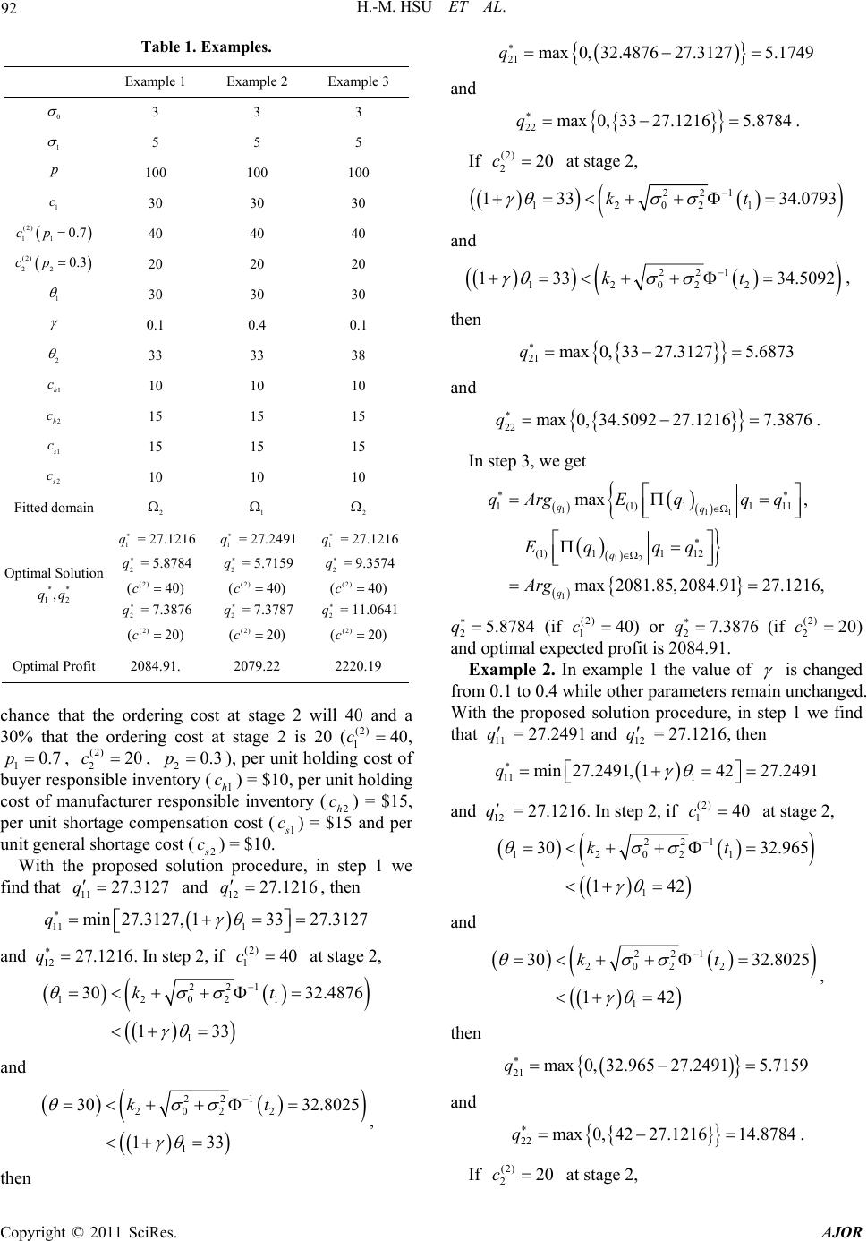 92 H.-M. HSU ET AL. Table 1. Examples. Example 1 Example 2 Example 3 0 3 3 3 1 5 5 5 100 100 100 1 c 30 30 30 (2) 11 0.7cp 40 40 40 (2) 22 0.3cp 20 20 20 1 30 30 30 0.1 0.4 0.1 2 33 33 38 1h c 10 10 10 2h c 15 15 15 1 c 15 15 15 2 c 10 10 10 Fitted domain 2 1 2 Optimal Solution ** 12 ,qq 1 q = 27.1216 2 = 5.8784 q () (2) 40c 2 = 7.3876 q () (2) 20c 1 q = 27.2491 2 q = 5.7159 () (2) 40c 2 q = 7.3787 () (2) 20c 1 q = 27.1216 2 = 9.3574 q ((2) 40c ) 2 = 11.0641q ((2)20c ) Optimal Profit 2084.91. 2079.22 2220.19 chance that the ordering cost at stage 2 will 40 and a 30% that the ordering cost at stage 2 is 20 ((2) 140c , 1, , 2), per unit holding cost of buyer responsible inventory (1h) = $10, per unit holding cost of manufacturer responsible inventory (2h) = $15, per unit shortage compensation cost ( 0.7p(2) 220c0.3pcc 1 c) = $15 and per unit general shortage cost (2 c) = $10. With the proposed solution procedure, in step 1 we find that and , then 11 27.3127q12 27.1216q 11 1 min27.3127, 13327.3127q and . In step 2, if at stage 2, 12 27.1216q(2) 140c 221 12021 1 30 32.4876 133 kt and 221 202 2 1 30 32.8025 133 kt , then 21 max0,32.487627.31275.1749q and 22 max0, 3327.12165.8784q. If (2) 220c at stage 2, 221 12021 1 3334.0793kt and 221 12022 1 3334.5092kt , then 21 max0,3327.31275.6873q and 22 max0, 34.509227.12167.3876q. In step 3, we get 111 12 1 1(1)11 (1)11 12 max , max2081.85, 2084.9127.1216, qq q q qArgE qqq Eq qq Arg 11 2 (if 5.8784q(2) 14 c ) or 2 (if 7.3876q(2) 220c ) and optimal expected profit is 2084.91. Example 2. In example 1 the value of is changed from 0.1 to 0.4 while other parameters remain unchanged. With the proposed solution procedure, in step 1 we find that 11 q = 27.2491 and 12 q = 27.1216, then 11 1 min27.2491, 14227.2491q and 12 q = 27.1216. In step 2, if at stage 2, (2) 140c 221 12021 1 30 32.965 142 kt and 221 202 2 1 30 32.8025 142 kt , then 21 max0,32.96527.24915.7159q and 22 max 0, 4227.121614.8784q. If (2) 220c at stage 2, Copyright © 2011 SciRes. AJOR  H.-M. HSU ET AL. 93 221 12021 1 30( )34.6278 142 kt and 221 202 21 34.5092142kt , then 21 max0,34.627827.24917.3787q and 22 max 0, 4227.121614.8784q . In step 3, we get 111 12 1 1(1)11 (1)1112 max , max2079.22,1846.8127.2491, qq q q qArgE qqq Eq qq Arg 11 2 (if ) or 2 (if 5.7159q(2) 140c7.3787q(2) 220c ) and optimal expected profit is 2079.22. Example 3. In example 1 the value of 2 is changed from 33 to 38 while other parameters remain unchanged. With the proposed solution procedure, in step 1 we find that = 27.4702 and = 27.1216, then 11 q12 q 11 1 min27.4702, 14227.4702q and = 27.1216. In step 2, if at stage 2, 12 q(2) 140c 221 12021 1 3335.7675kt and 221 12022 1 3336.479kt , then 21 max0, 3327.47025.5298q and 22 max0, 36.47927.12169.3574q . If at stage 2, (2) 220c 221 12021 1 3337.3228kt and 221 12022 1 3338.1857kt , then 21 max0,3327.47025.5298q and 22 max0, 38.185727.121611.0641q. In step 3, we get 111 12 1 1(1)11 (1)1112 max , max2131.75, 2220.1927.1216, qq q q qArgE qqq Eq qq Arg 11 2 (if 9.35 74q(2) 140c ) or 11.0641 (if (2) 220c ) and optimal expected profit is 2220.19. 3.2. Sensitivity Analysis 2 is an observation of 22 10 1 ,N at stage 2. At stage 1 we don’t know what value of 2 will be ob- served. With Monte Carlo method we randomly generate 100 values of 2 from 22 10 1 ,N , denoted as () 2 i , 1, ,100.i () 1 i q With the proposed solution procedure, we can find with respect to () 2 i . Then we evaluate the average expected profit value for using in 100 val- ues of () 1 i q () 2 i . The steps of Monte Carlo method are stated as follows: Step 1: Randomly generate () 2 i , from 1, ,100i 22 10 1 ,N . Step 2: With each () 2 i we can find by Proposi- tion 5, () 1 i q 1, ,100i respectively. Step 3: Compute the expected profit values for using () 1 i q in each () 2 i 1, ,100i , denoted as (1)( ) 1 i q , , )( ) 1 i q(100 (excluding 2 , parameters are fixed in () 1 ii qi () , 1,,100). Let *(1)() (2)()(100)() ()111100, 1, ,100. ii i iqq q i Step 4: optimal profit and optimal order quantity 1 q can be derived as follows: () 1 ** * 1(1) (2)(100) max,, , i q qArg . The relationships among optimal expected profit, short- age compensation range coefficient ( ), and buyer’s minimum-commitment quantity (1 ) are shown in Table 1 with the related parameters given in the illustrating example. And the relationships among optimal expected profit, shortage compensation range coefficient ( ) and shortage compensation cost 1 c, are shown in Table 2 and Table 3. In Table 2 we find that: 1) given 1 , we define the optimal expected profit turning point of decreasing as Copyright © 2011 SciRes. AJOR  94 H.-M. HSU ET AL. Table 2. Relationships among optimal expecte d profit, short- age compensation coefficient and buyer’s minimum-com- mitment quantity. 1 20 25 30 35 40 0 1836.02 2074.59 2345.81 2653.83 2990.32 0.1 1836.02 2074.59 2345.81 2653.83 2990.32 0.2 1836.02 2074.59 2345.81 2653.83 2990.32 0.3 1836.02 2074.59 2345.81 2653.83 2990.32 0.4 1836.02 2074.59 2345.81 2648.21 2985.97 0.5 1836.02 2067.19 2337.45 2645.42 2982.73 0.6 1832.17 2064.98 2335.56 2643.19 2980.85 0.7 1829.75 2064.86 2335.53 2643.11 2980.44 0.8 1829.53 2064.67 2335.47 2643.1 2980.41 0.9 1829.49 2064.65 2335.47 2643.1 2980.39 1 1829.48 2064.65 2335.45 2643.1 2980.39 Table 3. Relationships among optimal expecte d profit, short- age compensation coefficient and unit shortage compensa- tion cost (1) (given 1s c = 30). 1 c 15 30 45 60 75 0 2345.81 2345.81 2345.81 2345.81 2345.81 0.1 2345.81 2345.81 2345.81 2345.81 2345.81 0.2 2345.81 2345.81 2345.81 2345.81 2345.81 0.3 2345.81 2345.81 2345.81 2345.81 2345.81 0.4 2345.81 2345.81 2345.81 2345.81 2345.81 0.5 2337.45 2321.75 2312.85 2299.03 2270.26 0.6 2335.56 2315.03 2301.06 2283.1 2264.03 0.7 2335.53 2303.37 2290.98 2270.67 2243.73 0.8 2335.47 2302.57 2287.84 2266.5 2229.04 0.9 2335.47 2302.48 2286.71 2260.49 2228.85 1 2335.45 2302.47 2286.7 2260.49 2228.84 1 , that is, when 1 , the optimal expected profit is kept unchanged, but when 1 , the optimal expected profit decreases accordingly, i.e., 20 = 0.5, 25 = 30 = 0.4, 35 = 40 = 0.3. The larger 1 is, the smaller 1 is. 2) The marginal optimal expected profit is increased as 1 increases. In Table 3, Table 4 and Figure 3 with a given 1 we find that when 1 (30 = 0.4, 40 = 0.3), the optimal total order quantity 12 q is over q 1 1 which causes the shortage compensation cost can not be occurred. Hence, if 40 then the manu- facturer can give the buyer a larger shortage compensa- tion value of 1 c and take buyer’s increasing the value of 1 . For example, if the original shortage compensation coefficient = 0.2 and 1 = 30, then we find 30 = 0.4, the manufacturer can give = 0.3 and an arbitrarily large value of compensation cost 1 c to the buyer and take the buyer increasing the value of 1 from 30 to 40, then the optimal expected profit in the case of = 0.3 and 1 = 40 will be larger than it in the case of = 0.2 and 1 = 30. Base on the above description, the management in- sights observed from Table 2 to Table 4 can be con- cluded as follows: 1) The more the buyer’s minimum-commitment quan- tity 1 is, the more the expected profit of manufacturer is. 2) There are some ways to induce the buyer to in- crease the value of 1 : a) From Table 2, we know the upper bound of ( 1 ) which the manufacturer can give to the buyer to attract the buyer increasing the minimum commitment value of 1 without losing the expected profit. b) If the optimal total order quantity 12 is larger than q q 1 1 , then the manufacturer can give attractive values of shortage compensation cost 1 c (Tables 3 and 4) and shortage compensation coefficient ( ) (Table 2 to Table 4 to take buyer increasing the value of 1 . The manufacturer can provide alternatives for the buyer as Table 5 to induce the buyer to increase the value of 1 . Table 4. Relationships among optimal expecte d profit, short- age compensation coefficient and unit shortage compensa- tion cost (1) (given 1s c = 40). 1 c 15 30 45 60 75 0 2990.322990.322990.32 2990.32 2990.32 0.1 2990.322990.322990.32 2990.32 2990.32 0.2 2990.322990.322990.32 2990.32 2990.32 0.3 2990.322990.322990.32 2990.32 2990.32 0.4 2985.972963.112940.85 2934.03 2930.33 0.5 2982.732956.392932.06 2909.27 2887.73 0.6 2980.852952.732926.98 2903.1 2880.74 0.7 2980.442951.932925.84 2901.67 2879.04 0.8 2980.412951.842925.71 2901.5 2878.85 0.9 2980.392951.832925.7 2901.492878.84 1 2980.392951.832925.7 2901.492878.84 Copyright © 2011 SciRes. AJOR 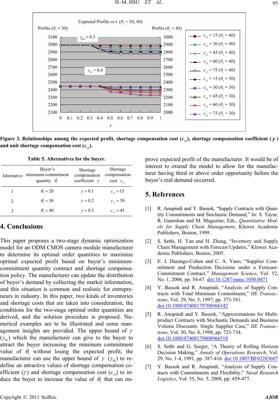 H.-M. HSU ET AL. Copyright © 2011 SciRes. AJOR 95 Figure 3. Relationships among the expected profit, shortage compensation cost (1), shortage compensation coefficient ( s c ) and unit shortage compe nsati on cost (1). s c Table 5. Alternatives for the buyer. Alternative Buyer’s minimum-commitment quantity 1 Shortage compensation coefficient Shortage compensation cost 1 c 1 120 0.1 115 s c 2 130 0.2 130 s c 3 140 0.3 145 s c 4. Conclusions This paper proposes a two-stage dynamic optimization model for an ODM CMOS camera module manufacturer to determine its optimal order quantities to maximize optimal expected profit based on buyer’s minimum- commitment quantity contract and shortage compensa- tion policy. The manufacturer can update the distribution of buyer’s demand by collecting the market information, and this situation is common and realistic for entrepre- neurs in industry. In this paper, two kinds of inventories and shortage costs that are taken into consideration, the conditions for the two-stage optimal order quantities are derived, and the solution procedure is proposed. Nu- merical examples are to be illustrated and some man- agement insights are provided. The upper bound of (1 ) which the manufacturer can give to the buyer to attract the buyer increasing the minimum commitment value of 1 without losing the expected profit, the manufacturer can use the upper bound of ( 1 ) to re- define an attractive values of shortage compensation co- efficient ( ) and shortage compensation cost (1 c) to in- duce the buyer to increase the value of 1 that can im- prove expected profit of the manufacturer. It would be of interest to extend the model to allow for the manufac- turer having third or above order opportunity before the buyer’s real demand occurred. 5. References [1] R. Anupindi and Y. Bassok, “Supply Contracts with Quan- tity Commitments and Stochastic Demand,” In: S. Tayur, R. Ganeshan and M. Magazine, Eds., Quantitative Mod- els for Supply Chain Management, Kluwer Academic Publishers, Boston, 1999. [2] S. Sethi, H. Yan and H. Zhang, “Inventory and Supply Chain Management with Forecast Updates,” Kluwer Aca- demic Publishers, Boston, 2005. [3] E. J. Durango-Cohen and C. A. Yano, “Supplier Com- mitment and Production Decisions under a Forecast- Commitment Contract,” Management Science, Vol. 52, No. 1, 2006, pp. 54-67. doi:10.1287/mnsc.1050.0471 [4] Y. Bassok and R. Anupindi, “Analysis of Supply Con- tracts with Total Minimum Commitment,” IIE Transac- tions, Vol. 29, No. 5, 1997, pp. 373-381. doi:10.1080/07408179708966342 [5] R. Anupindi and Y. Bassok, “Approximations for Multi- product Contracts with Stochastic Demands and Business Volume Discounts: Single Supplier Case,” IIE Transac- tions, Vol. 30, No. 8, 1998, pp. 723-734. doi:10.1080/07408179808966518 [6] S. Sethi and G. Sorger, “A Theory of Rolling Horizon Decision Making,” Annals of Operations Research, Vol. 29, No. 1-4, 1991, pp. 387-416. doi:10.1007/BF02283607 [7] Y. Bassok and R. Anupindi, “Analysis of Supply Con- tracts with Commitments and Flexibility,” Naval Research Logistics, Vol. 55, No. 5, 2008, pp. 459-477.  96 H.-M. HSU ET AL. doi:10.1002/nav.20300 [8] Z. Lian and A. Deshmukh, “Analysis of Supply Contracts with Quantity Flexibility,” European Journal of Opera- tional Research, Vol. 196, No. 2, 2009, pp. 526-533. doi:10.1016/j.ejor.2008.02.043 [9] G. Gallego and O. Ozer, “Integrating Replenishment Decisions with Advance Demand Information,” Man- agement Science, Vol. 47, No. 10, 2001, pp. 1344-1360. doi:10.1287/mnsc.47.10.1344.10261 [10] Y. Aviv, “A Time-Series Framework for Supply-Chain Inventory Management,” Operations Research, Vol. 51, No. 2, 2003, pp. 210-227. doi:10.1287/opre.51.2.210.12780 [11] A. Dvoretzky, J. Kiefer and J. Wolfowitz, “The Inventory Problem: II. Case of Unknown Distribution of Demand,” Econometrica, Vol. 20, No. 3, 1952, pp. 450-466. [12] H. Scarf, “Bayes Solution of the Statistical Inventory Problem,” Annals of Mathematical Statistics, Vol. 30, No. 2, 1959, pp. 490-508. doi:10.1214/aoms/1177706264 [13] H. Scarf, “Some Remarks on Bayes Solutions to the In- ventory Problem,” Naval Research Logistics, Vol. 7, No. 4, 1960, pp. 591-596. doi:10.1002/nav.3800070428 [14] M. A. Lariviere and E. L. Porteus, “Stalking Information: Bayesian Inventory Management with Unobserved Lost Sales,” Management Science, Vol. 45, No. 3, 1999, pp. 346-363. doi:10.1287/mnsc.45.3.346 [15] G. D. Eppen and A. V. Iyer, “Improved Fashion Buying with Bayesian Updates,” Operations Research, Vol. 45, No. 6, 1997, pp. 805-819. [16] J. Wu, “Quantity Flexibility Contracts under Bayesian Updating,” Computers & Operations Research, Vol. 32, No. 5, 2005, pp. 1267-1288. [17] A. V. Iyer and M. E. Bergen, “Quick Response in Manu- facturer-Retailer Channels,” Management Science, Vol. 43, No. 4, 1997, pp. 559-570. [18] T. M. Choi, D. Li and H. Yan, “Optimal Two-Stage Or- dering Policy with Bayesian Information Updating,” Jour- nal of the Operation Research Society, Vol. 54, No. 8, 2003, pp. 846-859. [19] O. Johnson and H. Thompson, “Optimality of Myopic Inventory Policies for Certain Dependent Demand Proc- esses,” Management Science, Vol. 21, No. 11, 1975, pp. 1303-1307. doi:10.1287/mnsc.21.11.1303 [20] W. H. Hausmann, “Sequential Decision Problems: A Model to Exploit Existing Forecast,” Management Science, Vol. 16, No. 2, 1969, pp. B93-B111. doi:10.1287/mnsc.16.2.B93 [21] D. Heath and P. Jackson, “Modeling the Evolution of Demand Forecast with Application to Safety Stock Ana- lysis in Production/Distribution Systems,” IIE Transac- tions, Vol. 26. No. 3, 1994, pp. 17-30. doi:10.1080/07408179408966604 [22] Y. Wang and B. Tomlin, “To Wait or Not to Wait: Opti- mal Ordering under Lead Time Uncertainty and Forecast Updating,” Naval Research Logistics, Vol. 56, No. 8, 2009, pp. 766-779. doi:10.1002/nav.20381 [23] H. Gurnani and C. S. Tang, “Optimal Ordering Decision with Uncertain Cost and Demand Forecast Updating,” Management Science, Vol. 45, No. 10, 1999, pp. 1456- 1462. doi:10.1287/mnsc.45.10.1456 [24] K. L. Donohue, “Efficient Supply Contract for Fashion Goods with Forecast Updating and Two Production Modes,” Management Science, Vol. 46, No. 11, 2000, pp. 1397- 1411. doi:10.1287/mnsc.46.11.1397.12088 [25] H. Y. Huang, S. Sethi and H. Yan, “Purchase Contract Management with Demand Forecast Updates,” IIE Transactions, Vol. 37, No. 8, 2005, pp. 775-785. doi:10.1080/07408170590961157 [26] H. Chen, J. Chen and Y. Chen, “A Coordination Mecha- nism for a Supply Chain with Demand Information Up- dating,” International Journal of Production Economics, Vol. 103, No. 1, 2006, pp. 347-361. doi:10.1016/j.ijpe.2005.09.002 [27] H. Yan, K. Liu and A. Hsu, “Order Quantity in Dual Supply Mode with Updating Forecasts,” Production and Operations Management, Vol. 12, No. 1, 2003, pp. 30-45. doi:10.1111/j.1937-5956.2003.tb00196.x [28] S. Sethi, H. Yan and H. Zhang, “Quantity Flexibility Contracts: Optimal Decisions with Information Updates,” Decision Sciences, Vol. 35, No. 4, 2004, pp. 691-712. doi:10.1111/j.1540-5915.2004.02873.x Copyright © 2011 SciRes. AJOR  H.-M. HSU ET AL. 97 Appendix A Proof of Proposition 1: 12 1 1 12 1 12 1 12 (2)212 , 222 1 (2) 22 12 dd dd dd qq h qq qq hs qq Eqq q pfxxc fxx cfxxcfxxc After rearranging the above equation, we have 12 1 (2)2 12 , (2) 2121212 1 dd 1 qq hs s Eqq q pcc FqqpcFc and 12 1 22 (2)2 12 , dd qq Eqq q 21212 . hs pccfq q If hold for , then 12 0 sh pc c2[0, )q 12 1 22 (2)212 , dd0 qq Eqq q . Therefore 12 1 (2)2 1,qq Eqq is concave for . The proof of 2[0, )q 12 (2)2 1,qq Eqq2 is the same as 12 1 (2)2 1,qq Eqq . Appendix B Proof of Proposition 2: For, let 1 12 (2)2 12 ,2 21212 (2) 12 1 10 qq hs s Eqq q pcc Fqqp cF c If 221 120211 1kt , 221 2120 21 1 max 0,qk t q , where (2) 1121 2 1 sh tpcFc pcc 1 s . If 221 202 1 1kt 1 1 , we take the upper bound of 1 1 instead of 221 202 1 kt , If 211 1 max0, 1qq 221 202 11 tk , we take the lower bound of 11 instead of 221 202 1 kt , 211 1 max 0,q q . The proof of 2 is the same as 1 . Appendix C Proof of Equations (20)-(25): From (18), when 221 210 21 kq t , we can know ; when 21 0q 221 210 21 kq t , . For given 21 0q Eq (2) 1,qc and , we can discuss with two 2 k 12 1 (1)1 ,qq conditions: 2, 2 0q0q and expected profit at stage 2 can be expressed as follows: 221 221 2 when 0,o qkq t 1 1221 221 22 12 11 1 1 221 22 2 202 1 221 202 1 2 1 (2)211 , 221 221 202 111220211 221 22011 0,d d dd d o kt qq hh kt kt h Eqq pfxxpxfxx Pktf x xcxf x xcktf x x cktxfxxc d 1 2 221 202 1 2 1 1 221 12021 (2) 2212222 21 202111202120 1 22 12222 21 02112021202 12112 d 1d 1 11 s kt shh hs ss hh s xktfxx cx fxxcktqpcck pcctc ck pc cck 2 22 021 (2)2 2 1211202 2 (2)2 2221 211202021 22 (2) 1112021 11 11 11 hhs hs s ccc ckk ccc kt ckcq Copyright © 2011 SciRes. AJOR  98 H.-M. HSU ET AL. 21 when 0,q 11 11 22 22 12 1 11 1 11 22 2 1 1 2 1 (2)21112 1 , 1 211211 1 22 22 21 21021202 1 0,d ddd dd d 1d q h qq q q hhs q shs h Eqqpfxx pxfxxpqfxxcxfxx cqfxxcqxfxxcxqfxx cx fxxpccqk pc 22 222222 12 02120212021202 22 22 12112021211202 22 11202112 1 11 11 11 hss hh sh s sh cqkcc k pcc ckcckq ckck 1 Therefore 1 113 1 2 12 1 12 1 12 12 1 113 1 (1)1(2)212 2 , ,1 (1) (2)21221 , 0, d 0, d nqddt iK qq qq i K qq qdd t EqpEqq fkk Eqq fkkcq By the same discussions, can be expressed as follows: 12 2 (1)1 ,qq Eq 221 22102 when 0,qkqt 2 1221 202 2 22 12 11 1 221 22 202 2 221 1202 2 2 2 1 (2)2112 2 , 221 202 211 221 221 22 022122 022 0,d d dd dd kt X qq h kt kt hh Eqq pfxxpxfxx pktfx xcxfx x ck tfxxck txfx x 2 221 202 2 221(2) 221 2 2202220221 2222221 12 02120222 022 (2)2 21(2) 121122220221 d s kt hhhs hh hhh cxk tfxxcktq pc ckpcct pc cc cckcctcq 22 when 0,q 11 22 2 12 2 11 1 11 2222 1 1 (2)2 111 , 112112121 22 2222 22 220212 0212021202 0,d dd ddd + q qq q q hhh s q hs hh Eqq pfxxpxfxxpqfxx cxfxxcqfxxcqxfxxcxqfxx pccq kpcck p d 12112 21hhh h cc ckcq Therefore Copyright © 2011 SciRes. AJOR  H.-M. HSU ET AL. Copyright © 2011 SciRes. AJOR 99 1 113 2 2 12 2 12 2 12 12 2 113 2 () (1)2 1(2)2122 , ,1 (1) (2)212 21 , 0, d 0, d nqdd t iK qq qq i K qq qdd t EqpEqq fkk Eqq fkkcq Appendix D In 2 , we redefine 122 (1) 111 , qq Eq qG q , if (2)(1) 0cc , (2) (1) 10Gq cc as 1 and q (1) 12 0 h Gqc c as 1 q, by the interme- diate value theorem, there exists a such 12 q[,] Proof of Proposition 4: In 1, we redefine 12 1 (1) 111 , qq Eq qG q . If (2)(1) 0cc, (2) (1) 10Gq cc as 1 and as 1, by the interme- diate value theorem, there exists a such q that 12 2 (1) 11 ,0 qq Eq q . If (2)(1) 0cc , (1) 11 0 h Gqc c q 11 q[, 10Gq as 1 and as 1, hence 1 q 10Gq q 0q when (2) (1) cc0 and this completes the proof. ] that 12 1 (1) 11 ,0 qq Eq q . If (2)(1) 0cc, 10Gq 1 q as 1 and as , hence when q 10Gq1 q 0(2) (1) cc0.
|