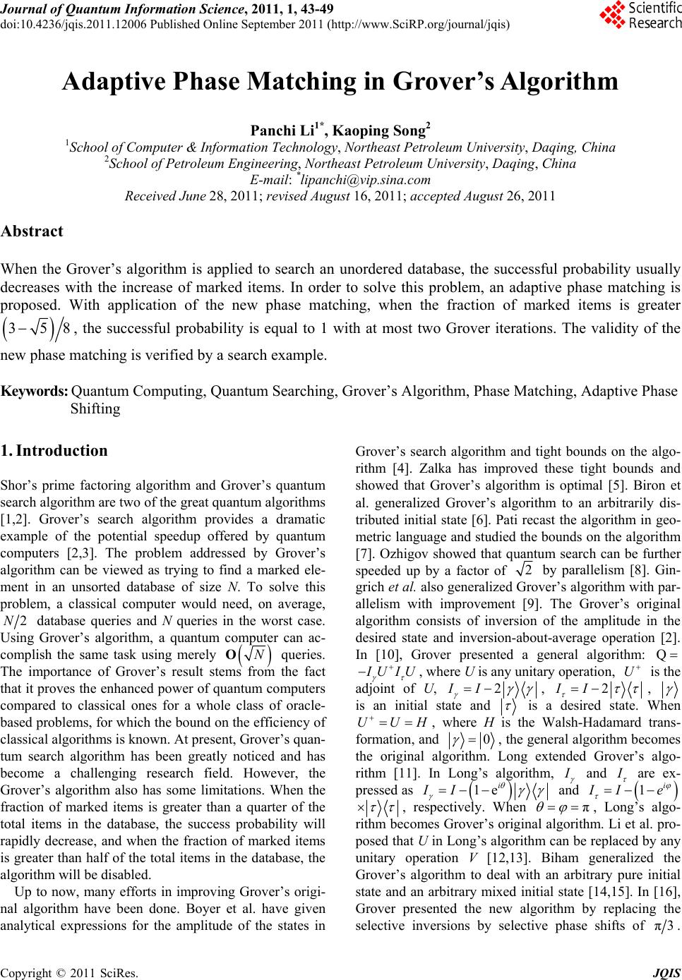
Journal of Quantum Informatio n Science, 2011, 1, 43-49
doi:10.4236/jqis.2011.12006 Published Online September 2011 (http://www.SciRP.org/journal/jqis)
Adaptive Phase Matching in Grover’s Algorithm
Panchi Li1*, Kaoping Song2
1School of Computer & Information Technology, Northeast Petroleum University, Daqing, China
2School of Petroleum Engineering, Northeast Petroleum University, Daqing, China
Received June 28, 2011; revised August 16, 2011; accepted August 26, 2011
Abstract
When the Grover’s algorithm is applied to search an unordered database, the successful probability usually
decreases with the increase of marked items. In order to solve this problem, an adaptive phase matching is
proposed. With application of the new phase matching, when the fraction of marked items is greater


358
, the successful probability is equal to 1 with at most two Grover iterations. The validity of the
new phase matching is verified by a search example.
Keywords: Quantum Computing, Quantum Searching, Grover’s Algorithm, Phase Matching, Adaptive Phase
Shifting
1. Introduction
Shor’s prime factoring algorithm and Grover’s quantum
search algorithm are two of the great quantum algorithms
[1,2]. Grover’s search algorithm provides a dramatic
example of the potential speedup offered by quantum
computers [2,3]. The problem addressed by Grover’s
algorithm can be viewed as trying to find a marked ele-
ment in an unsorted database of size N. To solve this
problem, a classical computer would need, on average,
2N database queries and N queries in the worst case.
Using Grover’s algorithm, a quantum computer can ac-
complish the same task using merely

NO

queries.
The importance of Grover’s result stems from the fact
that it proves the enhanced power of quantum computers
compared to classical ones for a whole class of oracle-
based problems, for which the bound on the efficiency of
classical algorithms is known. At present, Grover’s quan-
tum search algorithm has been greatly noticed and has
become a challenging research field. However, the
Grover’s algorithm also has some limitations. When the
fraction of marked items is greater than a quarter of the
total items in the database, the success probability will
rapidly decrease, and when the fraction of marked items
is greater than half of the total items in the database, the
algorithm will be disabled.
Up to now, many efforts in improving Grover’s origi-
nal algorithm have been done. Boyer et al. have given
analytical expressions for the amplitude of the states in
Grover’s search algorithm and tight bounds on the algo-
rithm [4]. Zalka has improved these tight bounds and
showed that Grover’s algorithm is optimal [5]. Biron et
al. generalized Grover’s algorithm to an arbitrarily dis-
tributed initial state [6]. Pati recast the algorithm in geo-
metric language and studied the bounds on the algorithm
[7]. Ozhigov showed that quantum search can be further
speeded up by a factor of 2 by parallelism [8]. Gin-
grich et al. also generalized Grover’s algorithm with par-
allelism with improvement [9]. The Grover’s original
algorithm consists of inversion of the amplitude in the
desired state and inversion-about-average operation [2].
In [10], Grover presented a general algorithm: Q

I
UIU


, where U is any unitary operation, U

is the
adjoint of U, 2II


  , 2II


  ,

is an initial state and

is a desired state. When
UU
H

, where H is the Walsh-Hadamard trans-
formation, and 0
 , the general algorithm becomes
the original algorithm. Long extended Grover’s algo-
rithm [11]. In Long’s algorithm,
I

and
I

are ex-
pressed as


1II

e
i 

 and


i
1
I
Ie




 , respectively. When π

 , Long’s algo-
mes Grover’s original algorithm. Li et al. pro-
posed that U in Long’s algorithm can be replaced by any
unitary operation V [12,13]. Biham generalized the
Grover’s algorithm to deal with an arbitrary pure initial
state and an arbitrary mixed initial state [14,15]. In [16],
Grover presented the new algorithm by replacing the
selective inversions by selective phase shifts of
rithm beco
π3.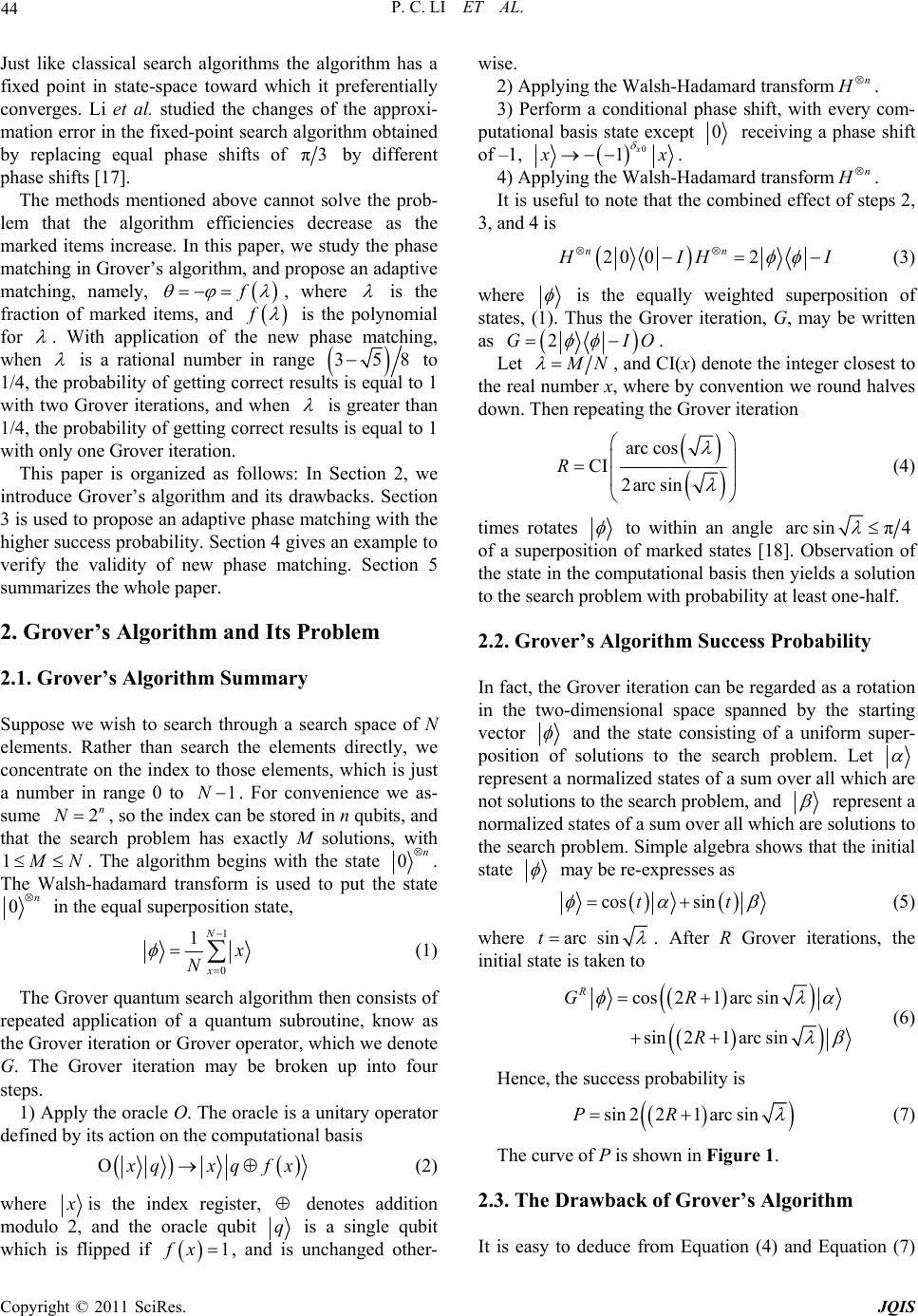

P. C. LI ET AL.
44
al sJust like classicearch algorithms the algorithm has a
fixed point in state-space toward which it preferentially
converges. Li et al. studied the changes of the approxi-
mation error in the fixed-point search algorithm obtained
by replacing equal phase shifts of π3 by different
phahifts [17]. se s
The methods mentioned above cannot solve the prob-
lem that the algorithm efficiencies decrease as the
marked items increase. In this paper, we study the phase
matching in Grover’s algorithm, and propose an adaptive
matching, namely, 
f

    , where

is the
fraction of marked items, and

f


is the polynomial
for

. With application of the new phase matching,
when

is a rational number in range

358 to
1/4, the probability of getting correct results is equal to 1
with two Grover iterations, and when

is greater than
1/4, the probability of getting correct results is equal to 1
with only one Grover iteration.
This paper is organized as follows: In Section 2, we
introduce Grover’s algorithm and its drawbacks. Section
3 is used to propose an adaptive phase matching with the
higher success probability. Section 4 gives an example to
verify the validity of new phase matching. Section 5
summarizes the whole paper.
2. Grover’s Algorithm and Its Problem
2.1. Grover’s Algorithm Summary
Suppose we wish to search through a search space of N
elements. Rather than search the elements directly, we
concentrate on the index to those elements, which is just
a number in range 0 to . For convenience we as-
sume , so the index can be stored in n qubits, and
that the search problem has exactly M solutions, with
1N
2n
N
1
M
N . The algorithm begins with the state 0n

.
The Walsh-hadamard transform is used to put the state
0n in the equal superposition state,
1
1N
0x
x
N




(1)
The Grover quantum search algorithm then consists of
repeated application of a quantum subroutine, know as
the Grover iteration or Grover operator, which we denote
G. The Grover iteration may be broken up into four
steps.
1) Apply the oracle O. The oracle is a unitary operator
defined by its action on the computational basis


O
x
qxqfx (2)
where
x
is the index register,  denotes addition
modulo 2, and the oracle qubit q is a single qubit
which is flipped if , and is unchanged other-
wise.

1fx
2) Applying the Walsh-Hadamard transformn
H

.
3) Perform a conditional phase shift, with every com-
putational basis state except 0 receiving a phase shift
of –1,

0
1x
x
x

 .
4) Applying the Walsh-Hadamard transformn
H

.
It is useful to note that the combined effect of steps 2,
3, and 4 is


20 02
nn
H
IH I 



(3)
where

is the equally weighted superposition of
states, (1). Thus the Grover iteration, G, may be written
as


2GI  O.
Let
M
N


, and CI(x) denote the integer closest to
the real number x, where by convention we round halves
down. Then repeating the Grover iteration



arc cos
CI
2arcsin
R








(4)
times rotates

to within an angle arc sinπ4  
of a superposition of marked states [18]. Observation of
the state in the computational basis then yields a solution
to the search problem with probability at least one-half.
2.2. Grover’s Algorithm Success Probability
In fact, the Grover iteration can be regarded as a rotation
in the two-dimensional space spanned by the starting
vector

and the state consisting of a uniform super-
position of solutions to the search problem. Let

represent a normalized states of a sum over all which are
not solutions to the search problem, and

represent a
normalized states of a sum over all which are solutions to
the search problem. Simple algebra shows that the initial
state

may be re-expresses as


cos sintt

   (5)
where arc sint

. After R Grover iterations, the
initial state is taken to





cos21arc sin
sin21arcsin
R
GR
R





 (6)
Hence, the success probability is



sin 221arcsinPR

 (7)
The curve of P is shown in Figure 1.
2.3. The Drawback of Grover’s Algorithm
It is easy to deduce from Equation (4) and Equation (7)

45 P. C. LI ET AL.
Figure 1. The success probability of Grover’s algorithm.
that when


35 80.14645,   P

decreases rap-
idly. When 0.146451 4,

 P

inceases rapidly. When r
14 12,

 P

decreases rapidly. When 12,


0R, P

there is

, and the algorithm is disabled.
Hence, the Grover's algorithm is no longer useful when
14

.
The reason for the problem is that the two phase rota-
tions in Grover iteration are fully equivalent in both am-
plitude and direction, namely . According to Ref. [18],
the result of such phase rotations is that, for the one Grover
iteration, the phase of the
π

increases 2arcsin

radians, and that rotating through at least arc cos

radians takes the

to

. When 35 ,1
8







,
there are only 1
1
4
  and 2
35
8


 make R an inte-
ger, namely, 1
1
1
arccos 1,
2arcsin
R


 2
2
2
arccos 2
2arcsin
R


 .
3. The Adaptive Phase Matching for
Grover’s Algorithm
3.1. The Adaptive Phase Matching
The two phase shift operators in the Grover’s algorithm
may be generally expressed as follows

1
1e
M
i
mm
m
UI




  (8)

1e e
i
V
i
I


  (9)
In the Grover’s original algorithm, there is π



.
According to the postulates of quantum mechanics [18],
the evolution of a closed quantum system is described by
a unitary transformation. So as far as the unitarity of op-
erators described by Equation (8) and Equation (9) is
concerned, we have the following conclusions.
Theorem 1 The operators described by Equation (8)
and Equation (9) are unitary.
Proof

1
U1e
M
i
m
I





 

 
11
2
1
2e e
1e1e
MM
ii
mm
M
ii
m
UU I
I








 


 




Hence, the operator described by Eqaution (8) is uni-
tary.



1
1e e
1e 1e
ee2
M
ii
m
ii
ii
VI
VV
I
I





 

 



 
 

 

Hence, the operator described by Equation (9) is uni-
tary.

For the matching of

and

, we propose an adap-
tive phase matching described by Theorem 2.
Theorem 2
1) When 14 1


 and 21 arc cos2

 


 

,
the success probability 1P

can be obtained after only
one iteration.
2) When 35 1
84



 and
35
arc cos14  


 



,
the success probability 1

P
can be obtained after only
two iterations.
Proof 1) For

described by Equation (1), applying
one Grover iteration gives

13
1
jk
UVA xB x
N
  
where


1
0
eee
NM i
ii
j
A
MN


 

M









1
0
ee1
Miii
k
BNM Me







 




Let



ee1pNM Me
iii 



 , the success
probability P is equal to


2
3.Mp When N,





P. C. LI ET AL.
46
using some simple algebra gives 32 812 4

 


32 32
8124cos48 5.

    cos When



212

 , namely,
 
arc cos212

  ，


2
32
32
max 32
812 4
485 1
43 4
PP

 

 
.
From cos 1
 , the range 14 1

 may be ob-
tained.
2) Reapplying one Grover iteration to 1

gives

21
5
1
jk
UVA xB x
N
  
where


 










1
0
1
0
22
1e e
11e1e
1e e
11e1e
eee
eeee
NM ii
j
ii
Mii
k
i
i
ii
ii
ii
ANC
NMCM D
BND
i
M
DNM C
CM NM
DNM M






 










 




  

 



D
Let





1e e11e
1
ii i
i
pNDM
NMe C
 

 
 
the success probability P is equal to

2
5
Mp N.
Where

  , use some simple algebra gives
 



5445433
54322
5432
5432
16 16cos64 11248cos
9624018844cos
6420823210012cos
1664925613 .
P





 
 
  


where 35 cos1 4 


 , max 1PP

.
From cos 1
 , the range


358  1 may be
obtained. Taking into account the only iteration is needed
when 14 1

, hence, the range for

takes the form

358 1  4, and the adaptive phase matching
takes the form
 
arc cos1354

  . □
According to thorem 2, applying the adaptive phase
matching, the Equation (8) and Equation (9) can be re-
expressed as follows

1
1e
M
i
m
UI




  (10)


V1e e
iI i




 

(11)
On the basis of the adaptive phase matching, the suc-
cess probability curve is shown in Figure 2.
3.2. The Algorithm Description Based on the
Adaptive Phase Matching
According to

, we divide the search process into three
cases.
1) When


035   8, the original phase
matching is applied.
2) When


358 1  4
create the phase of
, the adaptive phase
matching is applied. The search process can be described
as follows:
Step 1 Applying Equation (10) to
the marked states rotate




arc cos4354

 
radians, namely, 1U

 .
Step 2 Applying Equation (11) to rotate the system
superposition state 1

to 1

, namely, 11 V




1
VU

.
Step 3 Reapplying Equation (10) to 1

, namely,
2

1
U

.
Step 4 Reapplying Equation (11) to 2

, namely,
2



21
VVU

  .
Step 5 Measuring 2

.
3) When 14 1


, the adaptive phase matching is
applied. The search process can be described as fol-
lows:
Figure 2. Comparison of success probability curves between
Grover’s original algorithm and improved ones, where




1arc cos212,

 



2arc cos1354.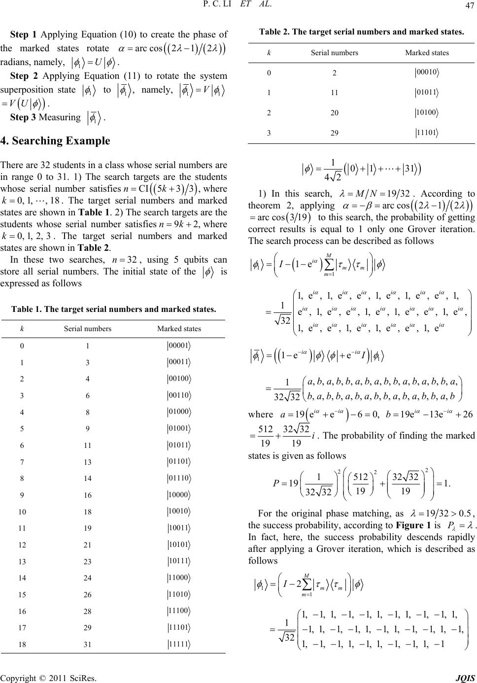
 

P. C. LI ET AL. 47
Step 1 Applying Equation (10) to create the phase o
the marked states rotate
f




arc cos212

 
Te 2. The mbers anes.
Serial bers Marked states
radians, namely, 1U

 .
Step 2 Applying Equation
superposition stat
(11) to rotate the system
e 1

to 1,

namely, 11 V

 

VU

.
Step 3 Measuring 1

.
4. Searching Example
ss whose serial numbers are
range 0 to 31. 1) The search targets are the students
There are 32 students in a cla
in
whose serial number satisfies
 
CI533 ,nk where
0, 1,, 18k. The target serial numbers and marked
states are shown in Table 1 . 2) are the
serial number satisfies 92,nk where
0, 1,2,3k. The target serial numbers and marked
states are shown in Table 2.
wo searches, 32n
The search targets
In these t
students whose

, using 5 qubits can
store all serial numbers. The initial state of the

is
ex
erial numbers and marked states.
pressed as follows
Table 1. The target s
k Serial numbers Marked states
0 1 00001
1 3 00011
2 4 00100
3 6 00110
4 8 01000
5 9 01001
6 11 01011
7 13 01101
8 14 01110
9 16 10000
abltarget serial nud marked stat
k num
0 2 00010
01011
1 11
2 20 10100
3 29 11101

101 31
42
 
1) In this search, 19 32MN


. According to
eorem 2, applyingth


 
arc cos212

  


arc cos3 19
correct
to this search, the probability of getting
results is equal to 1 only one Grover iteration.
Th described as foe search process can bellows

10 18 10010
11 19 10011
12 21 10101
13 23 10111
14 24 11000
15 26 11010
16 28 11100
17 29 11101
18 31 11111


1
11
, 1,
1
e,1,e,e,1,e,1,e,e,1,e,
32 1,e,e,1,e,1,e,e,1,e
1e e
,,,,,,,,,,,
1
32 32
i
iiiiiii
ii i ii i
ii
I
I
ababba b abb a
















 
,,,,,
,,,,,,,,,,,,,,,
babba
babbababbababbab



where
1
1e
1,e,1,e,e ,1,e ,1,e,e
M
i
mm
m
iiiii










19 ee60,
ii
a
 

 19e 13e26
ii
b
 
 
51232 32
1919 i . The probability of finding the marked
states is given as follows
2
22
151232 32
19 1.
19 19
32

32
P







  

matching, as



For the original phase 19 320.5

,
gure 1 is P the success probability, according to Fi



.
ds rapidly In fact, here, the success probability descen
after applying a Grover iteration, which is described as
follows
1
1
2
M
mm
m
I 





1, 1,1, 1, 1,1, 1,1, 1, 1,1,
1
1,1,1,1,1,1,1,1,1,1,1,
32 1, 1,1,1, 1,1, 1, 1,1,1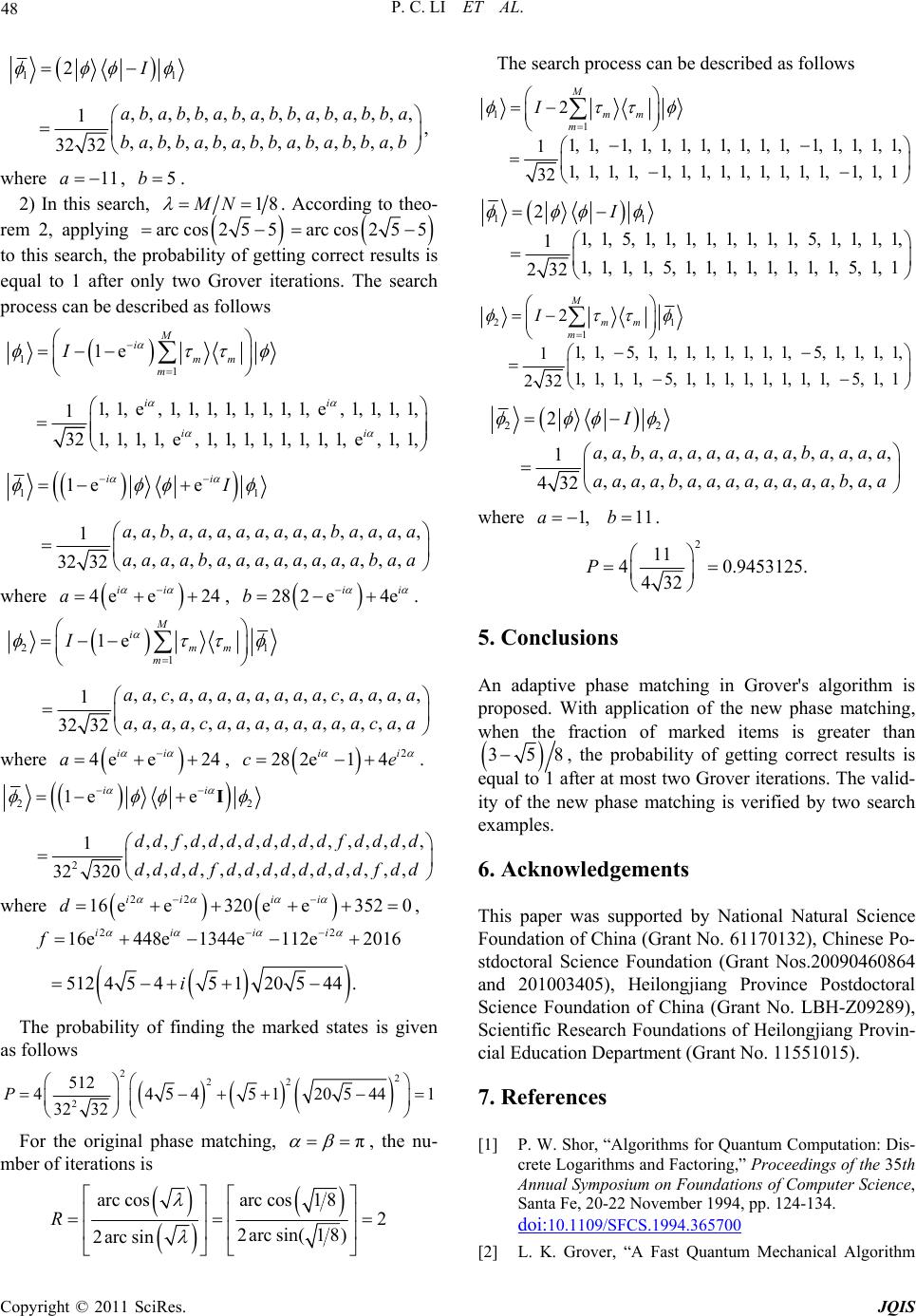
 





 




P. C. LI ET AL.
48

11
2
,,,,,,,,,,,,,,,,
1
,
,, ,,,,,,,, ,,,,,
32 32
I
ababbababbababba
babbababbababbab
 




where
2) In this search,
11a , 5b.
18MN

. According to theo-
rem 2, applying

arc cos255


arc cos255
getting correct results is to this search, the probability of
equal to 1 after only two Grover iterations. The search
process can be described as follows



1
i





1
11
1e
,,,,,,,,,,,,,,,,
1
,,,,,,,,,,
32 32
M
mm
ii
I
aabaaaaaaaabaaaa
aaaabaaaaaa




 


,,,,,aabaa



where
1, 1,e, 1, 1, 1, 1, 1, 1, 1, 1,e, 1, 1, 1, 1,
1
321, 1, 1, 1,e, 1, 1, 1, 1, 1, 1, 1, 1,e, 1, 1,
1e e
m
ii
ii
I


 






 


4e e24
ii
a
 
,

28 2e4e
ii
b

 
.

21
1
1e
,,,,,,,,,,,,,,,,
1
,,,,,,,,,,,,,,,
32 32
M
i
mm
m
I
aacaaaaaaaacaaaa
aaaacaaaaaaaacaa











where ,

4e e24
ii
a
 


2
28 2e14
ii
ce


.


22
2
1ee
,,,,,,,,,,,,,,,,
1
,,,,,,,,,,,,,,,
32 320
ii  
ddf ddddddddf dddd
ddddf ddddddddf dd
  



I
where 

22
16 ee320 ee3520
ii ii
d
  
,


2ii ii   2
16e448e 134112e2016
5124545120544.i
 

The probability of finding the marked states is given
as follows
4ef



22
22
2
512
445451 205441
32 32
P 
 
 
For the original phase matching, π

 
, the
mber of iterations is
nu-

 
arc cosarc cos1 8
R

 
 

 2
2arcsin(1 8)
2arcsin


 
 
The search process can be described as follows
1
1
1, 1, 1,
1
mm
m





2
1, 1, 1, 1, 1, 1, 1, 1,1, 1, 1, 1, 1,
1, 1, 1, 1,1, 1, 1, 1, 1, 1, 1, 1, 1,1, 1, 1
32
M
I 









11
2
1, 1,5, 1,1, 1,1, 1, 1,1, 1,5, 1,1, 1,1,
1
1, 1,1, 1,5, 1,1, 1, 1,1, 1,1, 1,5,
232


1, 1
I  



21
1
2
1, 1,5, 1, 1, 1, 1, 1, 1, 1, 1,5, 1, 1, 1, 1,
1
1, 1, 1, 1,5, 1, 1, 1, 1, 1, 1,1, 1,5, 1, 1
232
M
mm
m
I 













22
2
,,,,,,,,,,,,,,,,
1
,,,,,,,,,,,,,,,
432
I
aabaaaaaaaabaaaa
aaaabaaaaaaaabaa
 



1,a

 11b

. where
2
11
4 0.9453125.
432
P 


5. Conclusions
An adaptive phase matching in Grover's algorithm is
d. Witpplication of the new phase matching,
fraction ofarked items is greater than
proposeh a
when the m


35
equal
8, the probability of getting correct results is
to 1 after at most two Grover iterations. The valid-
y of the new phase matching is verified by two search
esearch Foundations of Heilongjiang Provin-
rant No. 11551015).
. References
it
examples.
6. Acknowledgements
This paper was supported by National Natural Science
Foundation of China (Grant No. 61170132), Chinese Po-
stdoctoral Science Foundation (Grant Nos.20090460864
and 201003405), Heilongjiang Province Postdoctoral
Science Foundation of China (Grant No. LBH-Z09289),
Scientific R
cial Education Department (G
7
[1] P. W. Shor, “Algorithms for Quantum Computation: Dis-
crete Logarithms and Factoring,” Proceedings of the 35th
Annual Symposium on Foundations of Computer Science,
Santa Fe, 20-22 November 1994, pp. 124-134.
doi:10.1109/SFCS.1994.365700
[2] L. K. Grover, “A Fast Quantum Mechanical Algorithm

P. C. LI ET AL.
49
ACM Symposium on the Theory of Computing, 1996, pp.
] L. K. Grover, “Quantum Mechanics Helps in Searching
for Database Search,” Proceedings of the 28th Annual
212-221.
[3
for a Needle in a Haystack,” Physical Review Letters, Vol.
79, No. 2, 1997, pp. 325-328.
doi:10.1103/PhysRevLett.79.325
[4] M. Boyer, G. Brassard, P. HØyer and A. Tapp
Bounds on Quantum Searching,”
, “Tight
Fortschritte Der Physik,
Vol. 46, No. 4-5, 1998, pp. 493-505.
doi:10.1002/(SICI)1521-3978(199806)46:4/5<493::AID-
PROP493>3.0.CO;2-P
[5] C. Zalka, “Grover’s Quantum Searching Algorithm Is
Optimal,” Physical Review A, Vol. 60, No. 4, 1999, pp.
2746-2751. doi:10.1103/PhysRevA.60.2746
[6] D. Biron, O. Biham, E. Biham,
“Generalized Grover Search Algorithm
M. Grassl and D. A. Lidar
for Arbitrar
rithm and Bounds
of Iterated Quantum Search by
Generalized
sing Any Transformation,” Physical Review Le
,
y Ini-
tial Amplitude Distribution,” quant-ph/9801066, 1998, pp.
1-8.
[7] A. K. Pati, “Fast Quantum Search Algo
on It,” quant-ph/9807067, 1998, pp. 1-4.
[8] Y. Ozhigov, “Speedup
Parallel Performance,” quant-ph/9904039, 1999, pp. 1-
21.
[9] R. Gingrich, C. P. Williams and N. Cerfm, “
Quantum Search with Parallelism,” quant-ph/9904039,
1999, pp. 1-14.
[10] L. K. Grover, “Quantum Computers Can Search Rapidly
by Utters,
Vol. 80, No. 19, 1998, pp. 4329-4332.
doi:10.1103/PhysRevLett.80.4329
[11] G. L. Long, Y. S. Li and W. L. Zhang, “Phase Matching
in Quantum Searching,” Physics Letters A, Vol. 262, No.
1, 1999, pp. 27-34. doi:10.1016/S0375-9601(99)00631-3
[12] D. F. Li and X. X. Li, “More General Quantu
Algorithm Q = –IVIU and the Pr
m Search
ecise Formula for the
γ τ
Amplitude and the Non-syssetric Effects of Different
Rotating Angles,” Physics Letters A, Vol. 287, No. 5-6,
2001, pp. 304-316.
doi:10.1016/S0375-9601(01)00498-4
[13] D. F. Li, X. X. Li and H. T. Huang, “Phase Condition for
the Grover Algorithm,” Theoretical and Mathematical
Physics, Vol. 144, No. 3, 2005, pp. 1279-1287.
doi:10.1007/s11232-005-0159-x
Grover’s Quantum [14] E. Biham, O. Biham and D. Birom, “
Search Algorithm for an Arbitrary Initial Amplitude Dis-
tribution,” Physical Review A, Vol. 60, No. 4, 1999, pp.
2742-2745. doi:10.1103/PhysRevA.60.2742
[15] E. Biham and D. Kenigsberg, “Grover’s Quantum Search
.
Press,
Algorithm for an Arbitrary Initial Mixed State,” Physical
Review A, Vol. 66, No. 6, 2002, pp. 1-4.
[16] L. K. Grover, “Fixed-Point Quantum Search,” Physical
Review Letters, Vol. 95, No. 15, 2005, pp. 1-4
[17] D. F. Li, X. R. Li, H. T. Huang and X. X. Li, “Fixed-
Point Quantum Search for Different Phase Shifts,” quant-
ph/0604062, 2006, pp. 1-8.
[18] M. A. Nielsen and I. L. Chuang, “Quantum Computation
and Quantum Information,” Cambridge University
Cambridge, 2000, pp. 248-255.