Wireless Sensor Network, 2009, 3, 222-232
doi:10.4236/wsn.2009.13029 ctober 2009 (http://www.SciRP.org/journal/wsn/).
Published Online O
An Adaptive Data Aggregation Algorithm in Wireless
Sensor Network with Bursty Source
Kumar PADMANABH, Sunil Kumar VUPPALA
Software Engineering and Technology Labs (SET Labs) Infosys Technologies Limited, Bangalore, India
Received April 20, 2009; revised May 25, 2009; accepted June 30, 2009
Abstract
The Wireless Sensor network is distributed event based systems that differ from conventional communica-
tion network. Sensor network has severe energy constraints, redundant low data rate, and many-to-one flows.
Aggregation is a technique to avoid redundant information to save energy and other resources. There are two
types of aggregations. In one of the aggregation many sensor data are embedded into single packet, thus
avoiding the unnecessary packet headers, this is called lossless aggregation. In the second case the sensor
data goes under statistical process (average, maximum, minimum) and results are communicated to the base
station, this is called lossy aggregation, because we cannot recover the original sensor data from the received
aggregated packet. The number of sensor data to be aggregated in a single packet is known as degree of ag-
gregation. The main contribution of this paper is to propose an algorithm which is adaptive to choose one of
the aggregations based on scenarios and degree of aggregation based on traffic. We are also suggesting a
suitable buffer management to offer best Quality of Service. Our initial experiment with NS-2 implementa-
tion shows significant energy savings by reducing the number of packets optimally at any given moment of
time.
Keywords: Data Aggregation, Data Fusion, Congestion Control, Buffer Overflow, End to End Delay
1. Introduction
Wireless sensor network (WSN) is a network of sensor
nodes. The main constituents of the WSN nodes are the
communication devices (i.e. receiver and transmitter), a
small Central Processing unit (CPU), a sensing device
and a battery. The sensor node senses and gathers infor-
mation from the surroundings; the CPU executes some
control instructions and the communication unit sends
the information to the base station through the network
of such a large number of nodes.
WSN is distributed in nature and an event based sys-
tem. Due to size and battery power limitations, these
devices typically have limited storage capacity, limited
energy resources, and limited network bandwidth. Due to
these limitations, WSN differs from traditional commu-
nication networks in several ways. These limitations of
sensor nodes demand specialized optimization tech-
niques. Typically in WSN applications, a large number
of Sensor Nodes (SNs) are covered over the specific tar-
get area in close proximity to each other. In such de-
ployments, spatial correlation of data is observed where
neighboring sensor nodes report data values with a high
degree of correlation.
Another kind of correlation observed in sensed envi-
ronmental data is the temporal correlation of data where
the successive sensed parameter values are found to be
identical and varies slowly except in the case of unex-
pected events [1,2].
The spatial and temporal correlations of the WSN data
can be exploited favorably for the development of effi-
cient communication protocols in the WSN. Moreover,
there is redundancy in the sensor data. The communica-
tion cost imposed due to redundant data is unnecessarily
consumes lifetime of the nodes and bandwidth. In wire-
less sensor networks, several information can be com-
bined together and represented by same number of bits.
Once this is done the energy consumption in the com-
munication process will be reduced. This process is
known as data aggregation. Data aggregation schemes
are the most popular way of using the correlation in sen-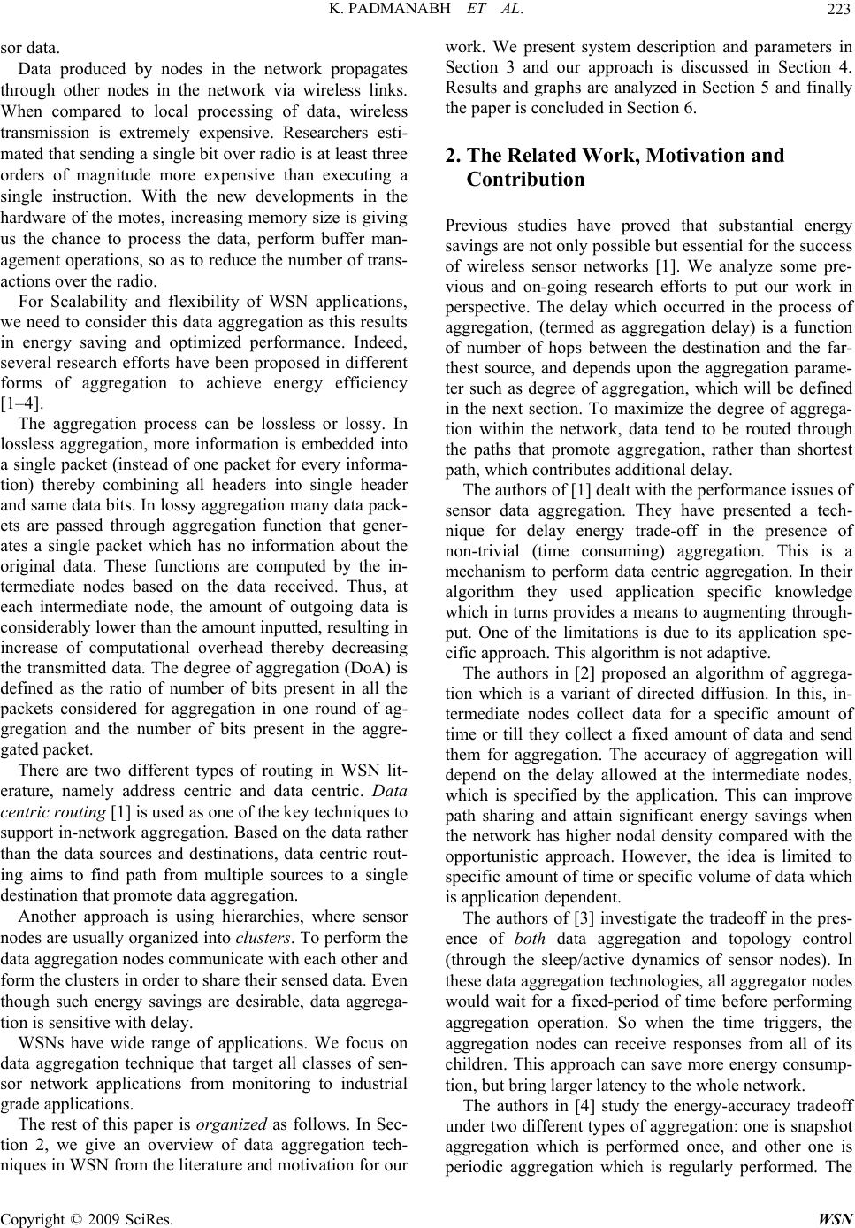

K. PADMANABH ET AL. 223
sor data.
Data produced by nodes in the network propagates
through other nodes in the network via wireless links.
When compared to local processing of data, wireless
transmission is extremely expensive. Researchers esti-
mated that sending a single bit over radio is at least three
orders of magnitude more expensive than executing a
single instruction. With the new developments in the
hardware of the motes, increasing memory size is giving
us the chance to process the data, perform buffer man-
agement operations, so as to reduce the number of trans-
actions over the radio.
For Scalability and flexibility of WSN applications,
we need to consider this data aggregation as this results
in energy saving and optimized performance. Indeed,
several research efforts have been proposed in different
forms of aggregation to achieve energy efficiency
[1–4].
The aggregation process can be lossless or lossy. In
lossless aggregation, more information is embedded into
a single packet (instead of one packet for every informa-
tion) thereby combining all headers into single header
and same data bits. In lossy aggregation many data pack-
ets are passed through aggregation function that gener-
ates a single packet which has no information about the
original data. These functions are computed by the in-
termediate nodes based on the data received. Thus, at
each intermediate node, the amount of outgoing data is
considerably lower than the amount inputted, resulting in
increase of computational overhead thereby decreasing
the transmitted data. The degree of aggregation (DoA) is
defined as the ratio of number of bits present in all the
packets considered for aggregation in one round of ag-
gregation and the number of bits present in the aggre-
gated packet.
There are two different types of routing in WSN lit-
erature, namely address centric and data centric. Data
centric routing [1] is used as one of the key techniques to
support in-network aggregation. Based on the data rather
than the data sources and destinations, data centric rout-
ing aims to find path from multiple sources to a single
destination that promote data aggregation.
Another approach is using hierarchies, where sensor
nodes are usually organized into clusters. To perform the
data aggregation nodes communicate with each other and
form the clusters in order to share their sensed data. Even
though such energy savings are desirable, data aggrega-
tion is sensitive with delay.
WSNs have wide range of applications. We focus on
data aggregation technique that target all classes of sen-
sor network applications from monitoring to industrial
grade applications.
The rest of this paper is organized as follows. In Sec-
tion 2, we give an overview of data aggregation tech-
niques in WSN from the literature and motivation for our
work. We present system description and parameters in
Section 3 and our approach is discussed in Section 4.
Results and graphs are analyzed in Section 5 and finally
the paper is concluded in Section 6.
2. The Related Work, Motivation and
Contribution
Previous studies have proved that substantial energy
savings are not only possible but essential for the success
of wireless sensor networks [1]. We analyze some pre-
vious and on-going research efforts to put our work in
perspective. The delay which occurred in the process of
aggregation, (termed as aggregation delay) is a function
of number of hops between the destination and the far-
thest source, and depends upon the aggregation parame-
ter such as degree of aggregation, which will be defined
in the next section. To maximize the degree of aggrega-
tion within the network, data tend to be routed through
the paths that promote aggregation, rather than shortest
path, which contributes additional delay.
The authors of [1] dealt with the performance issues of
sensor data aggregation. They have presented a tech-
nique for delay energy trade-off in the presence of
non-trivial (time consuming) aggregation. This is a
mechanism to perform data centric aggregation. In their
algorithm they used application specific knowledge
which in turns provides a means to augmenting through-
put. One of the limitations is due to its application spe-
cific approach. This algorithm is not adaptive.
The authors in [2] proposed an algorithm of aggrega-
tion which is a variant of directed diffusion. In this, in-
termediate nodes collect data for a specific amount of
time or till they collect a fixed amount of data and send
them for aggregation. The accuracy of aggregation will
depend on the delay allowed at the intermediate nodes,
which is specified by the application. This can improve
path sharing and attain significant energy savings when
the network has higher nodal density compared with the
opportunistic approach. However, the idea is limited to
specific amount of time or specific volume of data which
is application dependent.
The authors of [3] investigate the tradeoff in the pres-
ence of both data aggregation and topology control
(through the sleep/active dynamics of sensor nodes). In
these data aggregation technologies, all aggregator nodes
would wait for a fixed-period of time before performing
aggregation operation. So when the time triggers, the
aggregation nodes can receive responses from all of its
children. This approach can save more energy consump-
tion, but bring larger latency to the whole network.
The authors in [4] study the energy-accuracy tradeoff
under two different types of aggregation: one is snapshot
aggregation which is performed once, and other one is
periodic aggregation which is regularly performed. The
C opyright © 2009 SciRes. WSN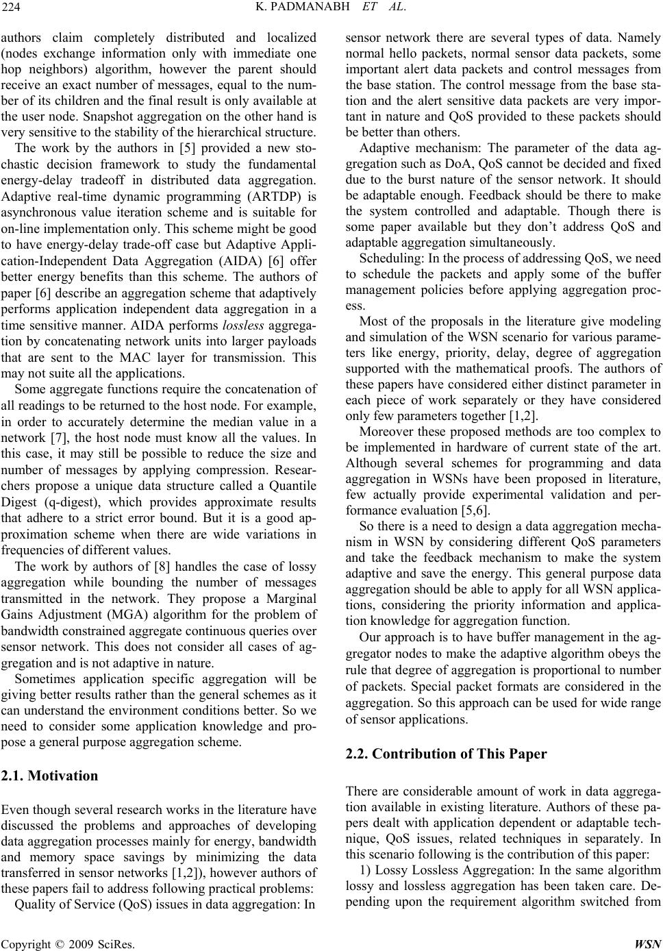

K. PADMANABH ET AL. 224
authors claim completely distributed and localized
(nodes exchange information only with immediate one
hop neighbors) algorithm, however the parent should
receive an exact number of messages, equal to the num-
ber of its children and the final result is only available at
the user node. Snapshot aggregation on the other hand is
very sensitive to the stability of the hierarchical structure.
The work by the authors in [5] provided a new sto-
chastic decision framework to study the fundamental
energy-delay tradeoff in distributed data aggregation.
Adaptive real-time dynamic programming (ARTDP) is
asynchronous value iteration scheme and is suitable for
on-line implementation only. This scheme might be good
to have energy-delay trade-off case but Adaptive Appli-
cation-Independent Data Aggregation (AIDA) [6] offer
better energy benefits than this scheme. The authors of
paper [6] describe an aggregation scheme that adaptively
performs application independent data aggregation in a
time sensitive manner. AIDA performs lossless aggrega-
tion by concatenating network units into larger payloads
that are sent to the MAC layer for transmission. This
may not suite all the applications.
Some aggregate functions require the concatenation of
all readings to be returned to the host node. For example,
in order to accurately determine the median value in a
network [7], the host node must know all the values. In
this case, it may still be possible to reduce the size and
number of messages by applying compression. Resear-
chers propose a unique data structure called a Quantile
Digest (q-digest), which provides approximate results
that adhere to a strict error bound. But it is a good ap-
proximation scheme when there are wide variations in
frequencies of different values.
The work by authors of [8] handles the case of lossy
aggregation while bounding the number of messages
transmitted in the network. They propose a Marginal
Gains Adjustment (MGA) algorithm for the problem of
bandwidth constrained aggregate continuous queries over
sensor network. This does not consider all cases of ag-
gregation and is not adaptive in nature.
Sometimes application specific aggregation will be
giving better results rather than the general schemes as it
can understand the environment conditions better. So we
need to consider some application knowledge and pro-
pose a general purpose aggregation scheme.
2.1. Motivation
Even though several research works in the literature have
discussed the problems and approaches of developing
data aggregation processes mainly for energy, bandwidth
and memory space savings by minimizing the data
transferred in sensor networks [1,2]), however authors of
these papers fail to address following practical problems:
Quality of Service (QoS) issues in data aggregation: In
sensor network there are several types of data. Namely
normal hello packets, normal sensor data packets, some
important alert data packets and control messages from
the base station. The control message from the base sta-
tion and the alert sensitive data packets are very impor-
tant in nature and QoS provided to these packets should
be better than others.
Adaptive mechanism: The parameter of the data ag-
gregation such as DoA, QoS cannot be decided and fixed
due to the burst nature of the sensor network. It should
be adaptable enough. Feedback should be there to make
the system controlled and adaptable. Though there is
some paper available but they don’t address QoS and
adaptable aggregation simultaneously.
Scheduling: In the process of addressing QoS, we need
to schedule the packets and apply some of the buffer
management policies before applying aggregation proc-
ess.
Most of the proposals in the literature give modeling
and simulation of the WSN scenario for various parame-
ters like energy, priority, delay, degree of aggregation
supported with the mathematical proofs. The authors of
these papers have considered either distinct parameter in
each piece of work separately or they have considered
only few parameters together [1,2].
Moreover these proposed methods are too complex to
be implemented in hardware of current state of the art.
Although several schemes for programming and data
aggregation in WSNs have been proposed in literature,
few actually provide experimental validation and per-
formance evaluation [5,6].
So there is a need to design a data aggregation mecha-
nism in WSN by considering different QoS parameters
and take the feedback mechanism to make the system
adaptive and save the energy. This general purpose data
aggregation should be able to apply for all WSN applica-
tions, considering the priority information and applica-
tion knowledge for aggregation function.
Our approach is to have buffer management in the ag-
gregator nodes to make the adaptive algorithm obeys the
rule that degree of aggregation is proportional to number
of packets. Special packet formats are considered in the
aggregation. So this approach can be used for wide range
of sensor applications.
2.2. Contribution of This Paper
There are considerable amount of work in data aggrega-
tion available in existing literature. Authors of these pa-
pers dealt with application dependent or adaptable tech-
nique, QoS issues, related techniques in separately. In
this scenario following is the contribution of this paper:
1) Lossy Lossless Aggregation: In the same algorithm
lossy and lossless aggregation has been taken care. De-
pending upon the requirement algorithm switched from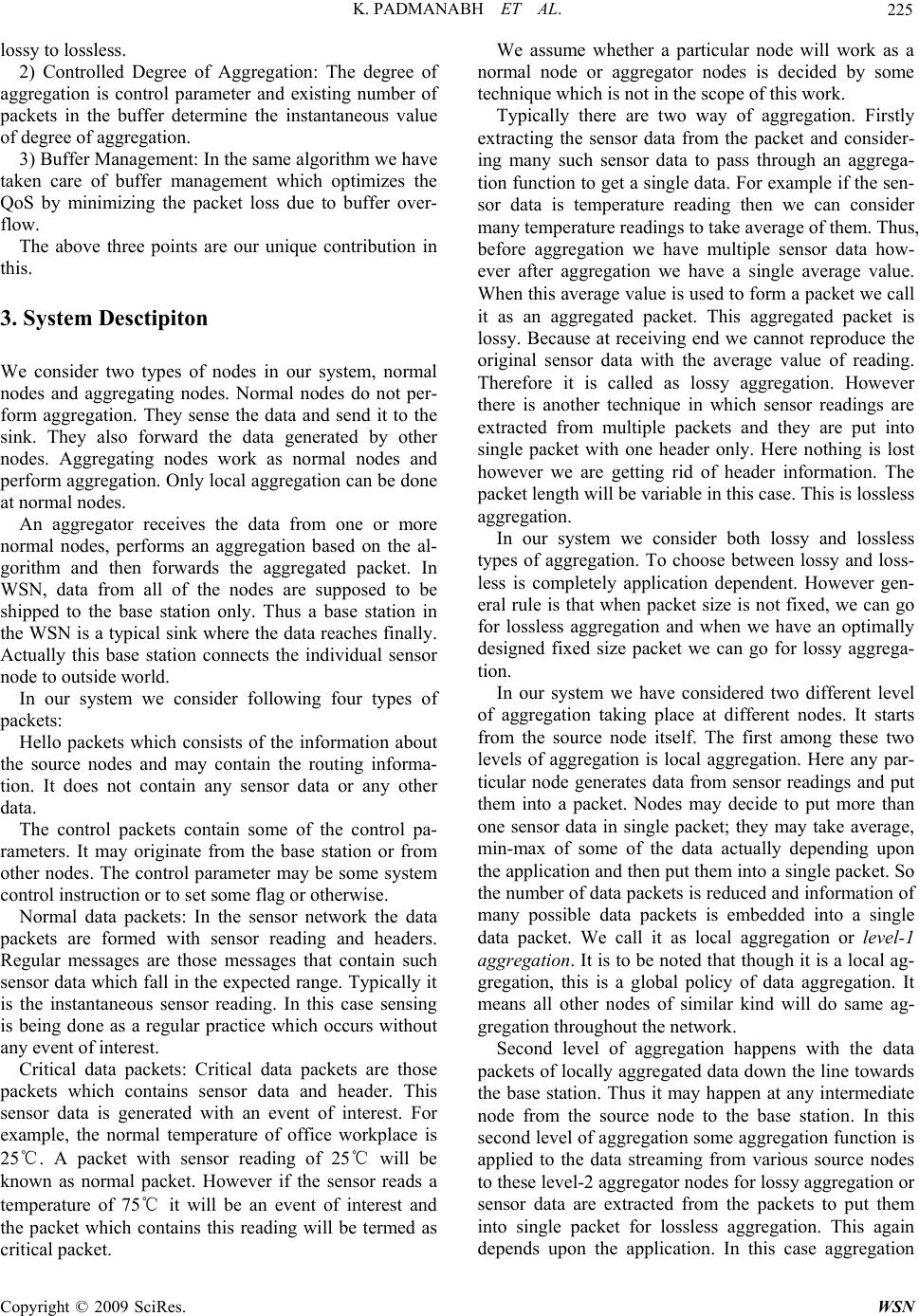

K. PADMANABH ET AL. 225
lossy to lossless.
2) Controlled Degree of Aggregation: The degree of
aggregation is control parameter and existing number of
packets in the buffer determine the instantaneous value
of degree of aggregation.
3) Buffer Management: In the same algorithm we have
taken care of buffer management which optimizes the
QoS by minimizing the packet loss due to buffer over-
flow.
The above three points are our unique contribution in
this.
3. System Desctipiton
We consider two types of nodes in our system, normal
nodes and aggregating nodes. Normal nodes do not per-
form aggregation. They sense the data and send it to the
sink. They also forward the data generated by other
nodes. Aggregating nodes work as normal nodes and
perform aggregation. Only local aggregation can be done
at normal nodes.
An aggregator receives the data from one or more
normal nodes, performs an aggregation based on the al-
gorithm and then forwards the aggregated packet. In
WSN, data from all of the nodes are supposed to be
shipped to the base station only. Thus a base station in
the WSN is a typical sink where the data reaches finally.
Actually this base station connects the individual sensor
node to outside world.
In our system we consider following four types of
packets:
Hello packets which consists of the information about
the source nodes and may contain the routing informa-
tion. It does not contain any sensor data or any other
data.
The control packets contain some of the control pa-
rameters. It may originate from the base station or from
other nodes. The control parameter may be some system
control instruction or to set some flag or otherwise.
Normal data packets: In the sensor network the data
packets are formed with sensor reading and headers.
Regular messages are those messages that contain such
sensor data which fall in the expected range. Typically it
is the instantaneous sensor reading. In this case sensing
is being done as a regular practice which occurs without
any event of interest.
Critical data packets: Critical data packets are those
packets which contains sensor data and header. This
sensor data is generated with an event of interest. For
example, the normal temperature of office workplace is
25 ℃. A packet with sensor reading of 25℃ will be
known as normal packet. However if the sensor reads a
temperature of 75℃ it will be an event of interest and
the packet which contains this reading will be termed as
critical packet.
We assume whether a particular node will work as a
normal node or aggregator nodes is decided by some
technique which is not in the scope of this work.
Typically there are two way of aggregation. Firstly
extracting the sensor data from the packet and consider-
ing many such sensor data to pass through an aggrega-
tion function to get a single data. For example if the sen-
sor data is temperature reading then we can consider
many temperature readings to take average of them. Thus,
before aggregation we have multiple sensor data how-
ever after aggregation we have a single average value.
When this average value is used to form a packet we call
it as an aggregated packet. This aggregated packet is
lossy. Because at receiving end we cannot reproduce the
original sensor data with the average value of reading.
Therefore it is called as lossy aggregation. However
there is another technique in which sensor readings are
extracted from multiple packets and they are put into
single packet with one header only. Here nothing is lost
however we are getting rid of header information. The
packet length will be variable in this case. This is lossless
aggregation.
In our system we consider both lossy and lossless
types of aggregation. To choose between lossy and loss-
less is completely application dependent. However gen-
eral rule is that when packet size is not fixed, we can go
for lossless aggregation and when we have an optimally
designed fixed size packet we can go for lossy aggrega-
tion.
In our system we have considered two different level
of aggregation taking place at different nodes. It starts
from the source node itself. The first among these two
levels of aggregation is local aggregation. Here any par-
ticular node generates data from sensor readings and put
them into a packet. Nodes may decide to put more than
one sensor data in single packet; they may take average,
min-max of some of the data actually depending upon
the application and then put them into a single packet. So
the number of data packets is reduced and information of
many possible data packets is embedded into a single
data packet. We call it as local aggregation or level-1
aggregation. It is to be noted that though it is a local ag-
gregation, this is a global policy of data aggregation. It
means all other nodes of similar kind will do same ag-
gregation throughout the network.
Second level of aggregation happens with the data
packets of locally aggregated data down the line towards
the base station. Thus it may happen at any intermediate
node from the source node to the base station. In this
second level of aggregation some aggregation function is
applied to the data streaming from various source nodes
to these level-2 aggregator nodes for lossy aggregation or
sensor data are extracted from the packets to put them
into single packet for lossless aggregation. This again
depends upon the application. In this case aggregation
C opyright © 2009 SciRes. WSN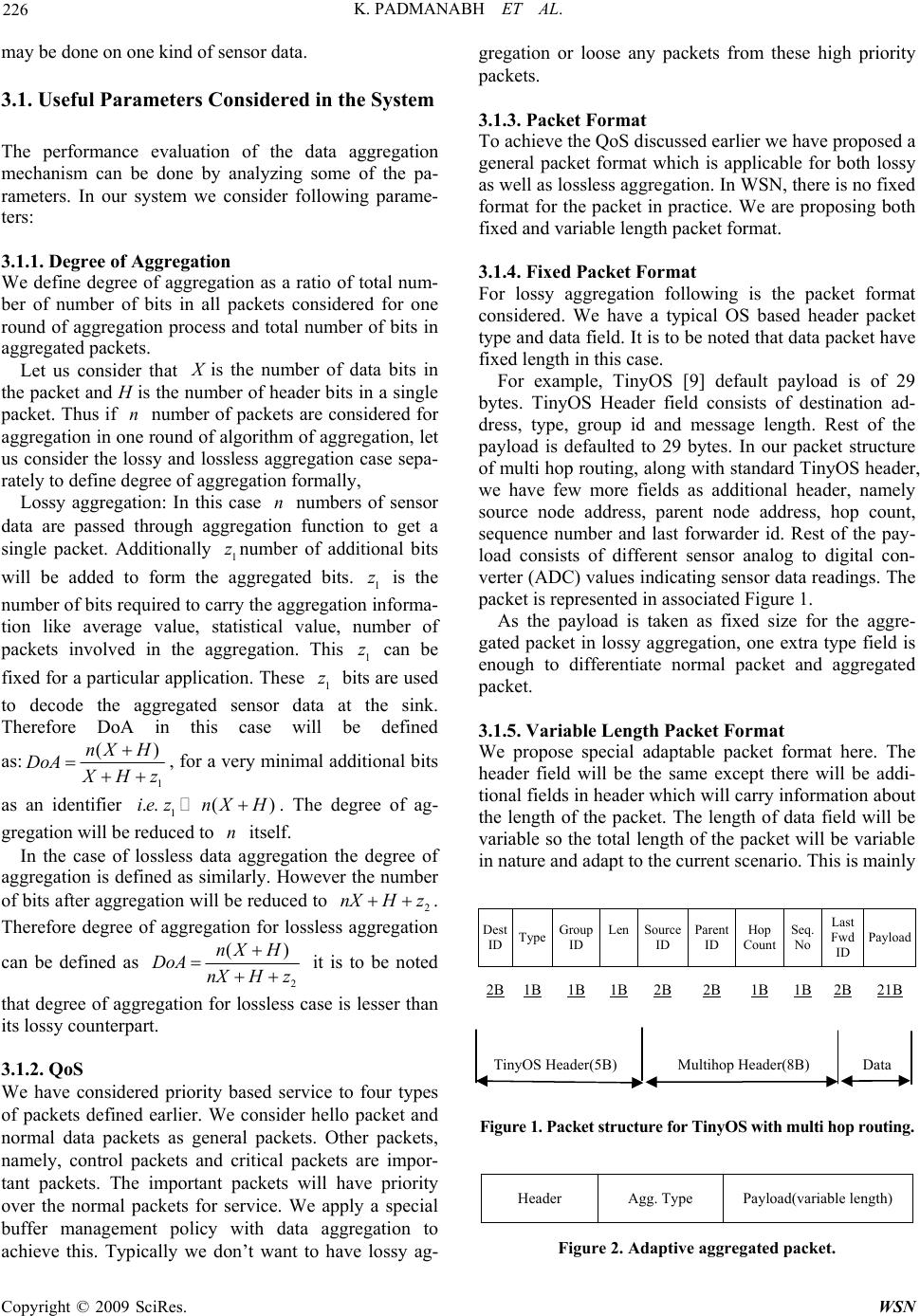

K. PADMANABH ET AL. 226
may be done on one kind of sensor data.
3.1. Useful Parameters Considered in the System
The performance evaluation of the data aggregation
mechanism can be done by analyzing some of the pa-
rameters. In our system we consider following parame-
ters:
3.1.1. Degree of Aggregation
We define degree of aggregation as a ratio of total num-
ber of number of bits in all packets considered for one
round of aggregation process and total number of bits in
aggregated packets.
Let us consider that
X
is the number of data bits in
the packet and H is the number of header bits in a single
packet. Thus if number of packets are considered for
aggregation in one round of algorithm of aggregation, let
us consider the lossy and lossless aggregation case sepa-
rately to define degree of aggregation formally,
n
Lossy aggregation: In this case numbers of sensor
data are passed through aggregation function to get a
single packet. Additionally number of additional bits
will be added to form the aggregated bits. is the
number of bits required to carry the aggregation informa-
tion like average value, statistical value, number of
packets involved in the aggregation. This can be
fixed for a particular application. These bits are used
to decode the aggregated sensor data at the sink.
Therefore DoA in this case will be defined
as:
n
1
z
1
z
1
z
1
z
1
(nX H
DoA )
X
Hz


, for a very minimal additional bits
as an identifier 1 ..ie znH(X)

. The degree of ag-
gregation will be reduced to itself. n
In the case of lossless data aggregation the degree of
aggregation is defined as similarly. However the number
of bits after aggregation will be reduced to 2
nX H z

.
Therefore degree of aggregation for lossless aggregation
can be defined as
2
(nX H
DoA nX H z

)

 it is to be noted
that degree of aggregation for lossless case is lesser than
its lossy counterpart.
3.1.2. QoS
We have considered priority based service to four types
of packets defined earlier. We consider hello packet and
normal data packets as general packets. Other packets,
namely, control packets and critical packets are impor-
tant packets. The important packets will have priority
over the normal packets for service. We apply a special
buffer management policy with data aggregation to
achieve this. Typically we don’t want to have lossy ag-
gregation or loose any packets from these high priority
packets.
3.1.3. Packet Format
To achieve the QoS discussed earlier we have proposed a
general packet format which is applicable for both lossy
as well as lossless aggregation. In WSN, there is no fixed
format for the packet in practice. We are proposing both
fixed and variable length packet format.
3.1.4. Fixed Packet Format
For lossy aggregation following is the packet format
considered. We have a typical OS based header packet
type and data field. It is to be noted that data packet have
fixed length in this case.
For example, TinyOS [9] default payload is of 29
bytes. TinyOS Header field consists of destination ad-
dress, type, group id and message length. Rest of the
payload is defaulted to 29 bytes. In our packet structure
of multi hop routing, along with standard TinyOS header,
we have few more fields as additional header, namely
source node address, parent node address, hop count,
sequence number and last forwarder id. Rest of the pay-
load consists of different sensor analog to digital con-
verter (ADC) values indicating sensor data readings. The
packet is represented in associated Figure 1.
As the payload is taken as fixed size for the aggre-
gated packet in lossy aggregation, one extra type field is
enough to differentiate normal packet and aggregated
packet.
3.1.5. Variable Length Packet Format
We propose special adaptable packet format here. The
header field will be the same except there will be addi-
tional fields in header which will carry information about
the length of the packet. The length of data field will be
variable so the total length of the packet will be variable
in nature and adapt to the current scenario. This is mainly
Dest
ID Type Group
ID
Len Source
ID
Parent
ID
Hop
Count
Seq.
No
Last
Fwd
ID
Payload
2B 1B1B 1B 2B 2B 1B 1B 2B 21B
TinyOS Header(5B) Multihop Header(8B) Data
Figure 1. Packet structure for TinyOS with multi hop routing.
Header Agg. Type Payload(variable length)
Figure 2. Adaptive aggregated packet.

K. PADMANABH ET AL. 227
Figure 3. Buffer and DoA relationship.
used for lossless aggregation. However it is to be noted
that there is a maximum limit to the length of this pay-
load. For example, in case of TinyOS, the message
length can be up to 116 bytes. So there will be different
combinations possible to prepare the variable aggregated
packet as sensor readings from different nodes need to be
sent in a single packet. We shall consider both the type
field in the header and the aggregation type in payload to
handle different combinations (Figure 2). This variable
packet needs to be interpreted correctly at the base sta-
tion by considering the aggregator type filed. By this
way, system can generate aggregated packet on the fly
based on the inputs given to the system.
3.1.6. Special Buffer Management for Data Aggregation
Data aggregation involves combining several sensor
readings in intermediate nodes. This in turn requires
storing the packets from different sensor nodes and
processes them in the memory space available in nodes
and outputting aggregated packet. To input the packets
from different sensor nodes, we consider buffer space in
the aggregator node and to process them we need a spe-
cial management policy [10,11] so that it can provide
specific number of packets to aggregation process after
considering type of packet and DoA type.
Buffer acts as a storage for the packets and works
similar to a queue. In our system, we consider a tempo-
rary buffer and multiple queue system in main buffer.
First the input packet reaches the temporary buffer and
then caters to different priority queues. We define dif-
ferent queues for different priority packets. For the first
queue in the buffer, we push normal and Type-1 critical
packets for which aggregation is needed. Second queue
is for important packets and third queue is for critical
packets. Let us consider that N is the total space in buffer
and B is the number of packets in the buffer (Figure 3).
Thus, F is considered as the difference between N and B
(i.e. N-B) indicating free space in the buffer [10].
The policy considered in the buffer management fol-
lows these rules.
1) General packet processing is on the first come first
serve basis.
2) From temporary buffer, the packet is pushed to
relevant queue in the main buffer based on the type of
packet.
3) A packet is never dropped as long as there is room
in the main buffer.
4) A packet from temporary buffer is discarded only if
the main buffer is full.
N
5) DoA is proportional to the number of packets (DOA
α B) as shown in the Figure 3.
6) If there is no space for incoming packet, packet of
the low priority is dropped from the temporary buffer.
F B
4. Our Approach
In this section, we present our approach of adaptive data
aggregation based on different parameters mentioned
earlier in the paper. In our system, aggregation is per-
formed in two levels after storing and processing the
sensor data packets in the buffer.
Hello packets and control packets are processed with-
out aggregation. Aggregation is performed for the nor-
mal packets. Based on the application demand, critical
data packets can also be aggregated. If the node can take
necessary action in response to the event of interest, we
may send the critical data packet after the aggregation,
referred as Type-1 critical packets. This is implemented
by incorporating necessary functionality inside the node.
For these Type-1 critical packets, a control packet is also
generated from the node. This control packet could be
sending an alarm signal or sending an alert to the corre-
sponding person. For Type-2 critical packets, no aggre-
gation takes place as the critical data packet is sent to the
sink as soon as possible. In this case, the sink responds to
the received critical data packet, which is generated for
the event of interest from the node.
The sensors sense the data at frequent intervals of time
and check for the possibility of any local aggregation
before generating the packets. This is referred to as local
aggregation. After local aggregation, the packet is gener-
ated and enters into the buffer of the next node towards
the sink from the input queue. Based on the aggregation
mechanism and type of packet, few packets are proc-
essed and an aggregated packet is outputted as described
in the algorithm. The effectiveness of data aggregation is
improved by taking feedback from the system. This
feedback contains the number of packets to be consid-
ered for aggregation in each round. We consider the
feedback and degree of aggregation type in the buffer
management to make adaptive aggregation as shown in
Figure 4.
Figure 4. Feedback mechanism in the data aggregation.
C opyright © 2009 SciRes. WSN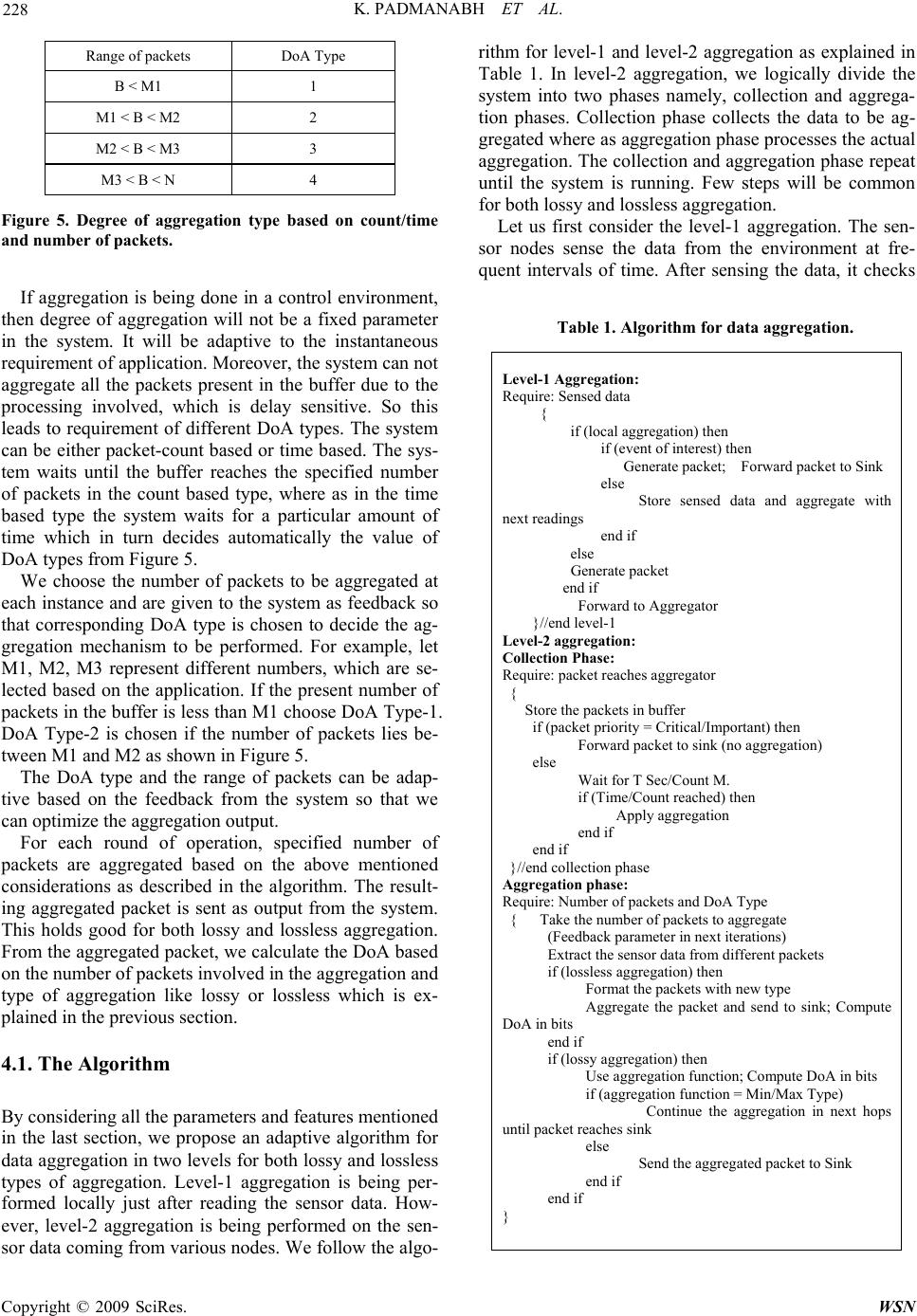

K. PADMANABH ET AL. 228
Range of packets DoA Type
B < M1 1
M1 < B < M2 2
M2 < B < M3 3
M3 < B < N 4
Figure 5. Degree of aggregation type based on count/time
and number of packets.
If aggregation is being done in a control environment,
then degree of aggregation will not be a fixed parameter
in the system. It will be adaptive to the instantaneous
requirement of application. Moreover, the system can not
aggregate all the packets present in the buffer due to the
processing involved, which is delay sensitive. So this
leads to requirement of different DoA types. The system
can be either packet-count based or time based. The sys-
tem waits until the buffer reaches the specified number
of packets in the count based type, where as in the time
based type the system waits for a particular amount of
time which in turn decides automatically the value of
DoA types from Figure 5.
We choose the number of packets to be aggregated at
each instance and are given to the system as feedback so
that corresponding DoA type is chosen to decide the ag-
gregation mechanism to be performed. For example, let
M1, M2, M3 represent different numbers, which are se-
lected based on the application. If the present number of
packets in the buffer is less than M1 choose DoA Type-1.
DoA Type-2 is chosen if the number of packets lies be-
tween M1 and M2 as shown in Figure 5.
The DoA type and the range of packets can be adap-
tive based on the feedback from the system so that we
can optimize the aggregation output.
For each round of operation, specified number of
packets are aggregated based on the above mentioned
considerations as described in the algorithm. The result-
ing aggregated packet is sent as output from the system.
This holds good for both lossy and lossless aggregation.
From the aggregated packet, we calculate the DoA based
on the number of packets involved in the aggregation and
type of aggregation like lossy or lossless which is ex-
plained in the previous section.
4.1. The Algorithm
By considering all the parameters and features mentioned
in the last section, we propose an adaptive algorithm for
data aggregation in two levels for both lossy and lossless
types of aggregation. Level-1 aggregation is being per-
formed locally just after reading the sensor data. How-
ever, level-2 aggregation is being performed on the sen-
sor data coming from various nodes. We follow the algo-
rithm for level-1 and level-2 aggregation as explained in
Table 1. In level-2 aggregation, we logically divide the
system into two phases namely, collection and aggrega-
tion phases. Collection phase collects the data to be ag-
gregated where as aggregation phase processes the actual
aggregation. The collection and aggregation phase repeat
until the system is running. Few steps will be common
for both lossy and lossless aggregation.
Let us first consider the level-1 aggregation. The sen-
sor nodes sense the data from the environment at fre-
quent intervals of time. After sensing the data, it checks
Table 1. Algorithm for data aggregation.
Level-1 Aggregation:
Require: Sensed data
{
if (local aggregation) then
if (event of interest) then
Generate packet; Forward packet to Sink
else
Store sensed data and aggregate with
next readings
end if
else
Generate packet
end if
Forward to Aggregator
}//end level-1
Level-2 aggregation:
Collection Phase:
Require: packet reaches aggregator
{
Store the packets in buffer
if (packet priority = Critical/Important) then
Forward packet to sink (no aggregation)
else
Wait for T Sec/Count M.
if (Time/Count reached) then
Apply aggregation
end if
end if
}//end collection phase
Aggregation phase:
Require: Number of packets and DoA Type
{ Take the number of packets to aggregate
(Feedback parameter in next iterations)
Extract the sensor data from different packets
if (lossless aggregation) then
Format the packets with new type
Aggregate the packet and send to sink; Compute
DoA in bits
end if
if (lossy aggregation) then
Use aggregation function; Compute DoA in bits
if (aggregation function = Min/Max Type)
Continue the aggregation in next hops
until packet reaches sink
else
Send the aggregated packet to Sink
end if
end if
}

K. PADMANABH ET AL. 229
for the need of any local aggregation (level-1) within the
node. If local aggregation is possible, it stores the sensor
data and waits for the next sensor readings before gener-
ating the packet. In case of any event of interest, the
packet is generated without waiting for local aggregation
and forwarded to the next node towards sink. Otherwise,
this node generates the packet and forwards it to the ag-
gregator node. If local aggregation is performed, it is
indicated by the type field in the packet format. So at this
point, several packets from different nodes reach the ag-
gregator nodes. This is referred as level-1 aggregation.
In the collection phase of level-2 aggregation, the ag-
gregator node collects the packets in the buffer. It checks
for the priority of the packets and append the packet in
the buffer as per the priority described in earlier section.
If the packet is found to be critical or important, they are
forwarded from the aggregator towards sink with out any
aggregation. In other words those packets are not aggre-
gated at all. In the system, it needs to identify either to
follow count based or time based mechanism for the ag-
gregation. In the count based, the system will wait for
specific number of incoming packets to be inserted into
the buffer. Then it aggregates the fixed number of pack-
ets (as per current DoA) from the head of the queue. The
choice of count based or time based depends on the ap-
plication.
Actually in phase-2, DoA type and number of packets
to be aggregated are taken as inputs. DoA type is taken
from predefined readings of the system as given in Fig-
ure 5. The number of packets to be aggregated at any
particular moment of time is determined by current space
in buffer which is taken as a feedback parameter as
shown in Figure 4. All these steps are similar for lossless
and lossy both. However, from this point onwards, lossy
and lossless aggregation methods differ and are de-
scribed as follows:
In lossy aggregation, particular number of packets in
buffer is considered for aggregation from the collection
phase and the sensor readings are extracted from differ-
ent packets. Then according to requirement of applica-
tion, a particular aggregation function is selected.
Basically there are two types of aggregation functions
possible. Functions like average, standard deviation are
limited to one hop only in aggregation process. That
means, once the packets are aggregated with this func-
tion, no further aggregation is suggested till it reaches the
sink. In the other case, functions like minimum, maxi-
mum can continue aggregation till it reaches to sink, fur-
ther reducing the number of packets transferred in the
system.
It is to be noted that except the type field for indication
of aggregated packet, the size of the packet remains same
in this case. At each aggregation step, the DoA is com-
puted in terms of bits. In our system we have considered
this for energy saving calculation and to analyze the sys-
tem performance.
In case of lossless aggregation, the sensor readings are
extracted from the packets taken from collection phase.
All these sensor readings are aggregated and formatted
into a packet with a new type and variable length. The
type and length fields describe the packet format to re-
trieve the readings at the sink. The DoA is computed in
terms of bits, at each aggregation step.
Once the packets with or without aggregation reach
the sink, it extracts the readings based on the packet type
and is used for the application. These steps are described
in the algorithm shown in Figure 6 and Table 1.
Figure 6. Flow chart of level-2 aggregation.
C opyright © 2009 SciRes. WSN

K. PADMANABH ET AL. 230
Different applications can be taken up to illustrate our
scheme. Let us consider temperature monitoring applica-
tion with average value as the aggregation function as
one illustrative application. This is a typical monitoring
application using sensor nodes. Nodes are deployed in a
room or in an open space where there is a need for
monitoring. The sink or base station is located either in
the same room where the nodes are deployed or in an-
other room. The packets carrying the sensor data reach
the base station in regular intervals of time. The base
station process the data and business logic is applied. So
the critical data packets should be sent to the base station
as soon as possible without the aggregation. Required
alerts are raised to the concerned person if the tempera-
ture readings are out of bound. Out of bound temperature
readings are considered as the event of interest. As the
aggregation function considered is average, the aggrega-
tion mechanism is considered up to 1 hop level only.
After the packets are aggregated, they are sent to sink
without further aggregation in the next levels.
In this application, the packet is generated every one
second at each node indicating the temperature reading.
If there is not much change in the sensor reading from
the previous value (up to a reference) we can do local
aggregation. After that the packets are generated and
reach the aggregator.
Based on the algorithm of lossy aggregation, packets
are aggregated and the aggregated packet is indicated as
a special type of packet. We follow the table (Figure 7)
to choose the DoA type.
Here it is a time based function. For every 10 seconds
the aggregation algorithm is called to check the number
of packets (B) and DoA type to apply the aggregation
mechanism in the system.
5. Analysis & Results
In this section we analyze the results from simulation of
our model. Different parameters considered in the system
are defined as follows:
Average Delay: Delay is taken as the time each packet
is in the buffer in the process of aggregation. Average
delay is calculated taking average time each packet
spends in the buffer.
Degree of Aggregation: The DoA is defined as the
ratio of number of bits present in all the packets consid-
ered for aggregation in one round of aggregation and the
number of bits present in aggregated packet.
Packet Loss: It indicates the number of packet drops
or loss due to buffering of the packets to aggregate in the
process of aggregation. Critical packets, important pack-
ets and normal packets are treated differently in the
buffer and corresponding loss rate is considered.
Range of packets Time DoA Type
B < 10 10 sec 1
10 < B < 20 10 sec 2
20 < B < 30 10 sec 3
30 < B < 100 10 sec 4
Figure 7. Example of time based DoA.
These parameters are considered for different Constant
Bit Rate traffic (CBR) traffic, network sizes in both lossy,
lossless aggregation based on count and time. We have
conducted simulations in Network Simulator (NS-2) [12]
to test the performance of our model in large scale.
Packet size is taken as 32 bytes, as described in earlier
section. Lossless aggregated packet size is variable and
maximum size is considered as 116 bytes. So each loss-
less aggregated packet can accommodate maximum of
20 packets considering 3 sensor readings per each packet.
CBR varies from 1 packet/sec to 40 packets/sec. Differ-
ent network sizes from 10 sensor nodes to 500 sensor
nodes are considered in the simulation. Buffer can ac-
commodate a total of 300 packets. For count based, 10
packets are aggregated at a time. In time based, we have
taken interval of 1 minute, so the number of packets dif-
fers as traffic and network size increases. This buffer is
divided into 3 equal parts (100 packets) for critical, im-
portant and normal packets. But this memory is sharable
among these packets giving the order of preferences, as
described in the system description of the paper.
5.1. Degree of Aggregation for Different
Network Sizes
Here DoA is considered for different network sizes as
shown in Figure 8 keeping the CBR as constant and
tested for all four possible combinations of lossless count
based, lossless time based, lossy count based and lossy
Figure 8. Degree of aggregation for different network sizes.

K. PADMANABH ET AL. 231
Figure 9. Degree of aggregation for different traffic.
Figure 10. Packet loss for different traffic.
Figure 11. Packet loss for different network sizes.
time based aggregations. In count based aggregation, the
DoA is in the range of 10 only both for lossy and lossless
due to the fact that as soon as count reaches for 10 pack-
ets, aggregation is applied. In case of time based aggre-
gation, DoA increases as network size increases based on
the table (Figure 5) for different DoA types. In case of
lossless aggregation, there is a limit of DoA as it can
accommodate maximum of 20 packets, so limiting the
DoA around 20. In the case of lossy aggregation, the
DoA grows as per the DoA type (Figure 5) and is limited
by the buffer size only. It is very evident that our pro-
posed algorithm makes the system adaptable to instanta-
neous condition and the required aggregated packet is
generated with proper DoA.
5.2. Degree of Aggregation for Different Traffic
Here DoA is considered for different traffic rates by
varying CBR flow as shown in Figure 9 keeping the net-
work size as constant of 100 nodes and tested for all four
possible combinations. In count based aggregation, the
DoA is in the range of 10 only both for lossy and lossless
due to the fact that count of 10 is the limit to trigger the
aggregation process. But DoA increases as traffic rate
increases in case of time based aggregation. In time
based lossless aggregation, DoA is around 20 as de-
scribed in the first graph. For lossy aggregation, DoA
increases as traffic load increases and grows as per the
DoA type. In this case, more packets are available for
aggregation with increase in traffic load. Only limitation
for DoA is the buffer size. Feedback is used at each stage
to choose the specific DoA type as mentioned in the al-
gorithm.
5.3. Packet Loss for Different Traffic and
Network Sizes
In our system, we have different types of packets (critical,
important and normal) which are treated differently in-
side the buffer in the process of aggregation. Our goal is
to minimize the loss of packets in the buffer and to have
less delay, for which a trade off is required. In Figure 10,
packet loss is shown for different traffic load keeping the
network size as constant at 100 nodes. In Figure 11,
packet loss is shown for different network sizes by
keeping the CBR as constant of 10 packets per sec. In
both the cases, loss of critical packets is very less ini-
tially but as network grows there are a bit of drop in the
critical packets. In case of the important packets and
normal packets also as traffic rate/network size increases,
there is a drop in the packets due to the limitation of
buffer size. But packet loss is more in time based when
compared to count based as the packets in the buffer are
limited in case of count based aggregation mechanism. In
count based, aggregation process is triggered by reaching
C opyright © 2009 SciRes. WSN

K. PADMANABH ET AL. 232
and makes the system adaptive to changes which can be
adjusted with the load in the buffer and buffer manage-
ment policy. The ultimate aim is to offer best QoS and
significant savings in the energy and number of packets
to be transmitted. The experiment has been carried out
with Network simulator for large scale sensor network
which advocates our proposed algorithm.
a specific number of packets in buffer even more packets
are generated in the system. In case of time based more
packets reach buffer as traffic load increases, so the loss
of packets. Overall, critical packets loss is very minimal,
as desired.
5.4. Average Delay for Different Network Sizes
7. References
Aggregation is applied more frequently in count based
therefore least delay is observed. In time based aggrega-
tion, more number of packets gets accumulated which is
resulted in more delay. However in lossy aggregation,
since the number of bits reduced drastically therefore,
least delay is there. In lossless aggregation no bits of
information is lost therefore more queuing delay is in-
troduced. This is why time based lossless aggregation
has highest delay. All four cases can be easily interpreted
from Figure 12.
[1] B. Krishnamachari, D. Estrin, and S. Wicker, “Modelling
data-centric routing in wireless sensor networks,” in Pro-
ceedings of the IEEE INFOCOM, 2002.
[2] C. Intanagonwiwat, D. Estrin, R. Govindan, and J. Hei-
demann, “Impact of network density on data aggregation
in wireless sensor networks,” in Proceedings of the 22nd
International Conference on Distributed Computing Sys-
tems (ICDCS’02), July 2002.
We need a tradeoff between the delay and the DoA
keeping the track of packet loss. Even though count
based aggregation is having less delay and less packet
loss rate, DoA is limited. But in case of time based ag-
gregation, we have better DoA at the cost of delay and
some packet loss. So lossy or lossless, count or time
based aggregation is to be chosen based on the applica-
tion type. Adaptive algorithm takes major role in getting
the increased DoA based on the feedback.
[3] V. Erramilli, I. Matta, and A. Bestavros , “On the interac-
tion between data aggregation and topology control in
wireless sensor networks,” First Annual IEEE Commu-
nications Society Conference on Sensor and Ad Hoc
Communications and Networks, IEEE SECON, pp.
557–565, 2004.
[4] A. Boulis, S. Ganeriwal, and M. B. Srivastava, “Aggre-
gation in sensor networks: An energy-accuracy trade-
off,” First IEEE International Workshop Sensor Network
Protocols and Applications (SNPA’03), May 2003.
6. Conclusions [5] Z. Ye, A. A. Abouzeid, and J. Ai, “Optimal policies for
distributed data aggregation in wireless sensor networks,”
in Proceedings of 26th Annual IEEE Conference on
Computer Communications (INFOCOM’07), Anchorage,
Alaska, USA, May 6–12, 2007.
The idea of the aggregation is to aggregate the data re-
quired close to the source or at intermediate nodes on the
way to sink instead of sending all the sensor readings
through the network. In this paper the idea of lossy and
lossless aggregation has been proposed within a single
algorithm. The proposed algorithm works for both lossy
and lossless aggregation depending upon the requirement
[6] T. He, B. Blum, J. Stankovic, and T. Abdelzaher, “AIDA:
Adaptive application independent data aggregation in
wireless sensor networks,” ACM Transaction on Sensor
Network, 2003.
[7] N. Shrivastava, C. Buragohain, D. Agrawal, and S. Suri,
“Medians and beyond: New aggregation techniques for
sensor networks,” in Proceedings of the Second ACM
Conference on Embedded Networked Sensor Systems
(SenSys’04), August 2004.
[8] A. Deligiannakis, Y. Kotidis, and Roussopoulos, “Band-
width-constrained queries in sensor networks,” The
VLDB Journal, Vol. 17, No. 3, pp. 443–467, 2008.
[9] TinyOS, http://www.tinyos.net/.
[10] K. Padmanabh and R. Roy, “Cost sensitive pushout pol-
icy and expelling polices with dynamic threshold for the
buffer management in differentiated service switch for
versatile traffic,” IEEE International Conference on Net-
working, Mauritius, April 23–28, 2006.
[11] G. J. Fosdhini and B. Gopinath, “Sharing memory opti-
mally,” IEEE Transaction on Communication, Vol. 31,
No. 3, pp. 352–360, March 1983.
Figure 12. Average delay in aggregation for different net-
work sizes. [12] Network Simulator 2, http://www.isi.edu/nsnam/ns/.