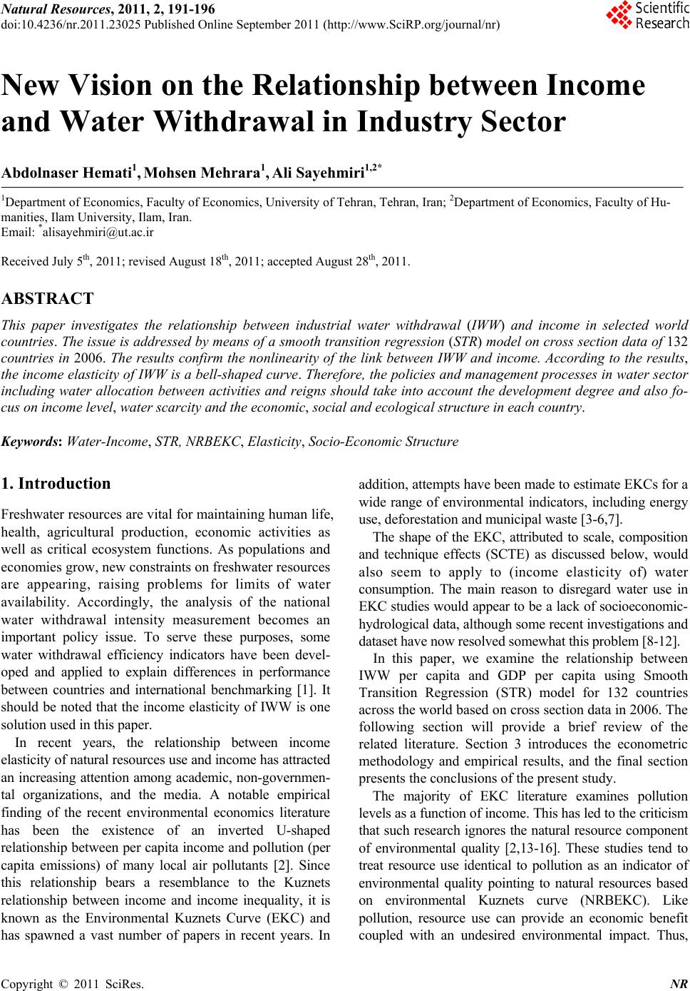
 Natural Resources, 2011, 2, 191-196 doi:10.4236/nr.2011.23025 Published Online September 2011 (http://www.SciRP.org/journal/nr) Copyright © 2011 SciRes. NR 191 New Vision on the Relationship between Income and Water Withdrawal in Industry Sector Abdolnaser Hemati1, Mohsen Mehrara1, Ali Sayehmiri1,2* 1Department of Economics, Faculty of Economics, University of Tehran, Tehran, Iran; 2Department of Economics, Faculty of Hu- manities, Ilam University, Ilam, Iran. Email: *alisayehmiri@ut.ac.ir Received July 5th, 2011; revised August 18th, 2011; accepted August 28th, 2011. ABSTRACT This paper investigates the relationship between industrial water withdrawal (IWW) and income in selected world countries. The issue is addressed by means of a smooth transition regression (STR) model on cross section data of 132 countries in 2006. The results confirm the nonlinearity of the link between IWW and income. According to the results, the income elasticity of IWW is a bell-shaped curve. Therefore, the policies and management processes in water sector including water allocation between activities and reigns should take into account the development degree and also fo- cus on income level, water scarcity and the economic, social and ecological structure in each country. Keywords: Water-Income, STR, NRBEKC, Elasticity, Socio-Economic Structure 1. Introduction Freshwater resources are vital for maintaining human life, health, agricultural production, economic activities as well as critical ecosystem functions. As populations and economies grow, new constraints on freshwater resources are appearing, raising problems for limits of water availability. Accordingly, the analysis of the national water withdrawal intensity measurement becomes an important policy issue. To serve these purposes, some water withdrawal efficiency indicators have been devel- oped and applied to explain differences in performance between countries and international benchmarking [1]. It should be noted that the income elasticity of IWW is one solution used in this paper. In recent years, the relationship between income elasticity of natural resources use and income has attracted an increasing attention among academic, non-governmen- tal organizations, and the media. A notable empirical finding of the recent environmental economics literature has been the existence of an inverted U-shaped relationship between per capita income and pollution (per capita emissions) of many local air pollutants [2]. Since this relationship bears a resemblance to the Kuznets relationship between income and income inequality, it is known as the Environmental Kuznets Curve (EKC) and has spawned a vast number of papers in recent years. In addition, attempts have been made to estimate EKCs for a wide range of environmental indicators, including energy use, deforestation and municipal waste [3-6,7]. The shape of the EKC, attributed to scale, composition and technique effects (SCTE) as discussed below, would also seem to apply to (income elasticity of) water consumption. The main reason to disregard water use in EKC studies would appear to be a lack of socioeconomic- hydrological data, although some recent investigations and dataset have now resolved somewhat this problem [8-12]. In this paper, we examine the relationship between IWW per capita and GDP per capita using Smooth Transition Regression (STR) model for 132 countries across the world based on cross section data in 2006. The following section will provide a brief review of the related literature. Section 3 introduces the econometric methodology and empirical results, and the final section presents the conclusions of the present study. The majority of EKC literature examines pollution levels as a function of income. This has led to the criticism that such research ignores the natural resource component of environmental quality [2,13-16]. These studies tend to treat resource use identical to pollution as an indicator of environmental quality pointing to natural resources based on environmental Kuznets curve (NRBEKC). Like pollution, resource use can provide an economic benefit coupled with an undesired environmental impact. Thus, 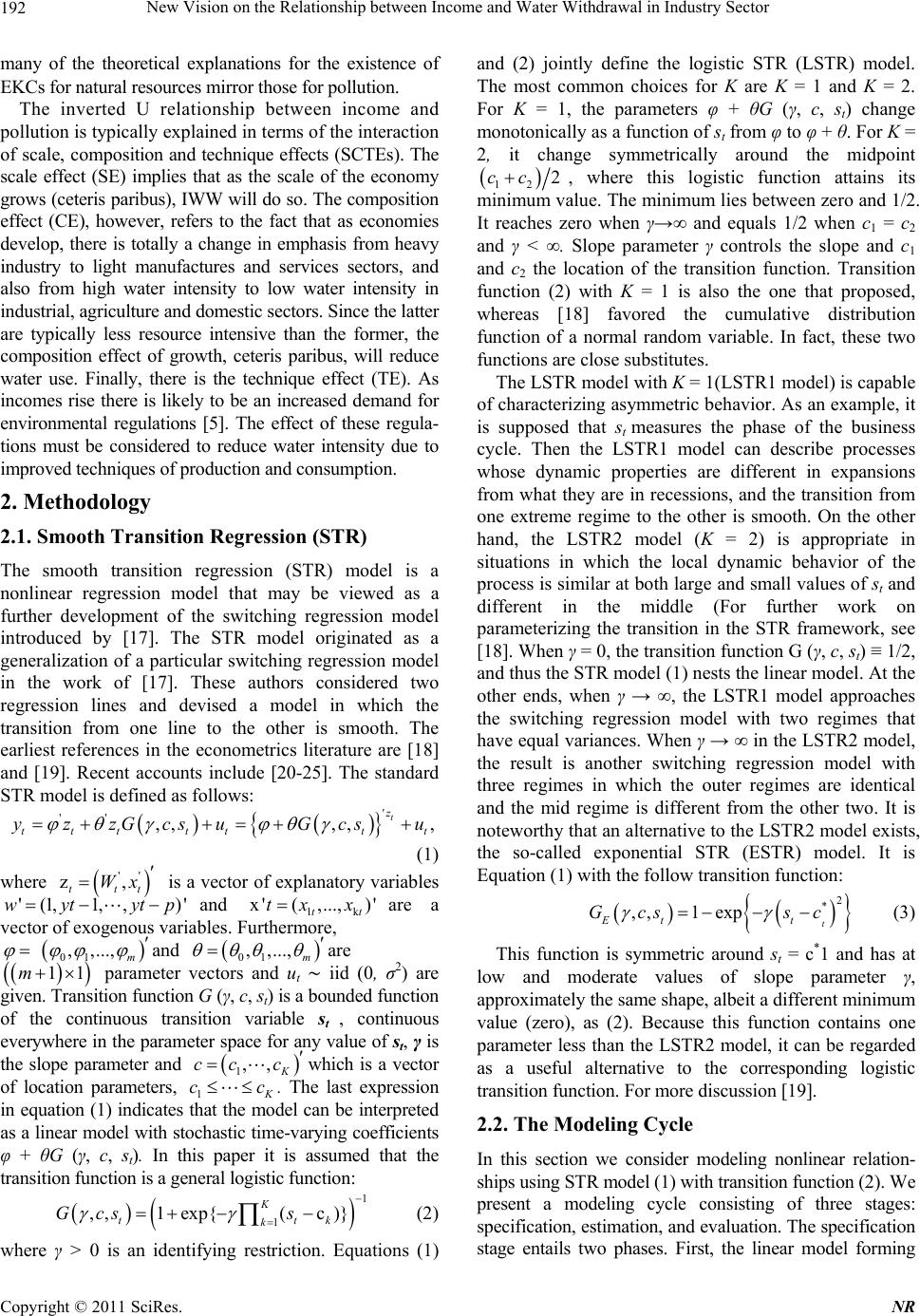 New Vision on the Relationship between Income and Water Withdrawal in Industry Sector 192 many of the theoretical explanations for the existence of EKCs for natural resources mirror those for pollution. The inverted U relationship between income and pollution is typically explained in terms of the interaction of scale, composition and technique effects (SCTEs). The scale effect (SE) implies that as the scale of the economy grows (ceteris paribus), IWW will do so. The composition effect (CE), however, refers to the fact that as economies develop, there is totally a change in emphasis from heavy industry to light manufactures and services sectors, and also from high water intensity to low water intensity in industrial, agriculture and domestic sectors. Since the latter are typically less resource intensive than the former, the composition effect of growth, ceteris paribus, will reduce water use. Finally, there is the technique effect (TE). As incomes rise there is likely to be an increased demand for environmental regulations [5]. The effect of these regula- tions must be considered to reduce water intensity due to improved techniques of production and consumption. 2. Methodology 2.1. Smooth Transition Regression (STR) The smooth transition regression (STR) model is a nonlinear regression model that may be viewed as a further development of the switching regression model introduced by [17]. The STR model originated as a generalization of a particular switching regression model in the work of [17]. These authors considered two regression lines and devised a model in which the transition from one line to the other is smooth. The earliest references in the econometrics literature are [18] and [19]. Recent accounts include [20-25]. The standard STR model is defined as follows: '' ',,,, , t tttttt t yzzGcsuGcs u '' z, ttt Wx (1) where is a vector of explanatory variables and 1are a vector of exogenous variables. Furthermore, '( )'p1, 1,,wyt yt 01 ,,...,m k x '(,...,)' tt tx x and 01 ,,..., m ,, K c are parameter vectors and ut iid (0, σ2) are given. Transition function G (γ, c, st) is a bounded function of the continuous transition variable st , continuous everywhere in the parameter space for any value of st, γ is the slope parameter and which is a vector of location parameters, 1 m 1 cc 11 cc. The last expression in equation (1) indicates that the model can be interpreted as a linear model with stochastic time-varying coefficients φ + θG (γ, c, st). In this paper it is assumed that the transition function is a general logistic function: 1 1 ,,1 exp{(c)} K tt k Gcs s k (2) where γ > 0 is an identifying restriction. Equations (1) and (2) jointly define the logistic STR (LSTR) model. The most common choices for K are K = 1 and K = 2. For K = 1, the parameters φ + θG (γ, c, st) change monotonically as a function of st from φ to φ + θ. For K = 2, it change symmetrically around the midpoint 12 2cc, where this logistic function attains its minimum value. The minimum lies between zero and 1/2. It reaches zero when γ→∞ and equals 1/2 when c1 = c2 and γ < ∞. Slope parameter γ controls the slope and c1 and c2 the location of the transition function. Transition function (2) with K = 1 is also the one that proposed, whereas [18] favored the cumulative distribution function of a normal random variable. In fact, these two functions are close substitutes. The LSTR model with K = 1(LSTR1 model) is capable of characterizing asymmetric behavior. As an example, it is supposed that st measures the phase of the business cycle. Then the LSTR1 model can describe processes whose dynamic properties are different in expansions from what they are in recessions, and the transition from one extreme regime to the other is smooth. On the other hand, the LSTR2 model (K = 2) is appropriate in situations in which the local dynamic behavior of the process is similar at both large and small values of st and different in the middle (For further work on parameterizing the transition in the STR framework, see [18]. When γ = 0, the transition function G (γ, c, st) ≡ 1/2, and thus the STR model (1) nests the linear model. At the other ends, when γ → ∞, the LSTR1 model approaches the switching regression model with two regimes that have equal variances. When γ → ∞ in the LSTR2 model, the result is another switching regression model with three regimes in which the outer regimes are identical and the mid regime is different from the other two. It is noteworthy that an alternative to the LSTR2 model exists, the so-called exponential STR (ESTR) model. It is Equation (1) with the follow transition function: 2 * ,,1 expt Et t Gcs sc (3) This function is symmetric around st = c*1 and has at low and moderate values of slope parameter γ, approximately the same shape, albeit a different minimum value (zero), as (2). Because this function contains one parameter less than the LSTR2 model, it can be regarded as a useful alternative to the corresponding logistic transition function. For more discussion [19]. 2.2. The Modeling Cycle In this section we consider modeling nonlinear relation- ships using STR model (1) with transition function (2). We present a modeling cycle consisting of three stages: specification, estimation, and evaluation. The specification stage entails two phases. First, the linear model forming Copyright © 2011 SciRes. NR 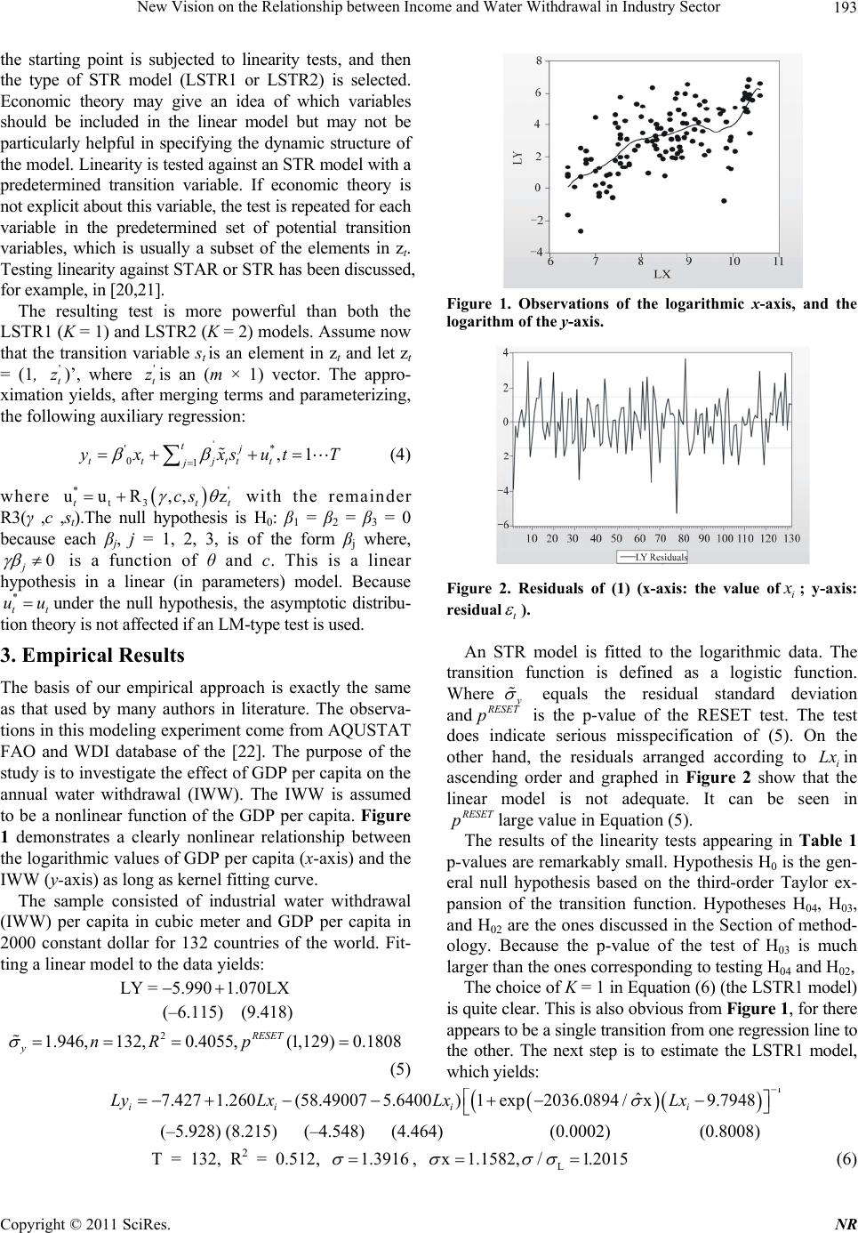 New Vision on the Relationship between Income and Water Withdrawal in Industry Sector Copyright © 2011 SciRes. NR 193 the starting point is subjected to linearity tests, and then the type of STR model (LSTR1 or LSTR2) is selected. Economic theory may give an idea of which variables should be included in the linear model but may not be particularly helpful in specifying the dynamic structure of the model. Linearity is tested against an STR model with a predetermined transition variable. If economic theory is not explicit about this variable, the test is repeated for each variable in the predetermined set of potential transition variables, which is usually a subset of the elements in zt. Testing linearity against STAR or STR has been discussed, for example, in [20,21]. Figure 1. Observations of the logarithmic x-axis, and the logarithm of the y-axis. The resulting test is more powerful than both the LSTR1 (K = 1) and LSTR2 (K = 2) models. Assume now that the transition variable st is an element in zt and let zt = (1, )’, where is an (m × 1) vector. The appro- ximation yields, after merging terms and parameterizing, the following auxiliary regression: ' t z' t z ' '* 01,1 tj tt jttt j yx xsutT (4) where tt * t3 ' uuR,,z t cs with the remainder R3(γ ,c ,st).The null hypothesis is H0: β1 = β2 = β3 = 0 because each βj, j = 1, 2, 3, is of the form βj where, 0 j * t uu is a function of θ and c. This is a linear hypothesis in a linear (in parameters) model. Because under the null hypothesis, the asymptotic distribu- t Figure 2. Residuals of (1) (x-axis: the value ofi ; y-axis: residualt ). tion theory is not affected if an LM-type test is used. An STR model is fitted to the logarithmic data. The transition function is defined as a logistic function. Where equals the residual standard deviation and ESET p is the p-value of the RESET test. The test does indicate serious misspecification of (5). On the other hand, the residuals arranged according to iin ascending order and graphed in Figure 2 show that the linear model is not adequate. It can be seen in Lx ESET plarge value in Equation (5). 3. Empirical Results The basis of our empirical approach is exactly the same as that used by many authors in literature. The observa- tions in this modeling experiment come from AQUSTAT FAO and WDI database of the [22]. The purpose of the study is to investigate the effect of GDP per capita on the annual water withdrawal (IWW). The IWW is assumed to be a nonlinear function of the GDP per capita. Figure 1 demonstrates a clearly nonlinear relationship between the logarithmic values of GDP per capita (x-axis) and the IWW (y-axis) as long as kernel fitting curve. The results of the linearity tests appearing in Table 1 p-values are remarkably small. Hypothesis H0 is the gen- eral null hypothesis based on the third-order Taylor ex- pansion of the transition function. Hypotheses H04, H03, and H02 are the ones discussed in the Section of method- ology. Because the p-value of the test of H03 is much larger than the ones corresponding to testing H04 and H02, The sample consisted of industrial water withdrawal (IWW) per capita in cubic meter and GDP per capita in 2000 constant dollar for 132 countries of the world. Fit- ting a linear model to the data yields: The choice of K = 1 in Equation (6) (the LSTR1 model) is quite clear. This is also obvious from Figure 1, for there appears to be a single transition from one regression line to the other. The next step is to estimate the LSTR1 model, which yields: LY =5.9901.070LX (–6.115) (9.418) 2 1.946,132,0.4055,(1,129) 0.1808 RESET ynR p (5) ˆ 7.427 1.260(58.490075.6400) 1 exp2036.0894/x9.7948 ii ii Ly LxLxLx (–5.928) (8.215) (–4.548) (4.464) (0.0002) (0.8008) T = 132, R2 = 0.512, 1.3916 , L x 1.1582.,/1 2015 (6) 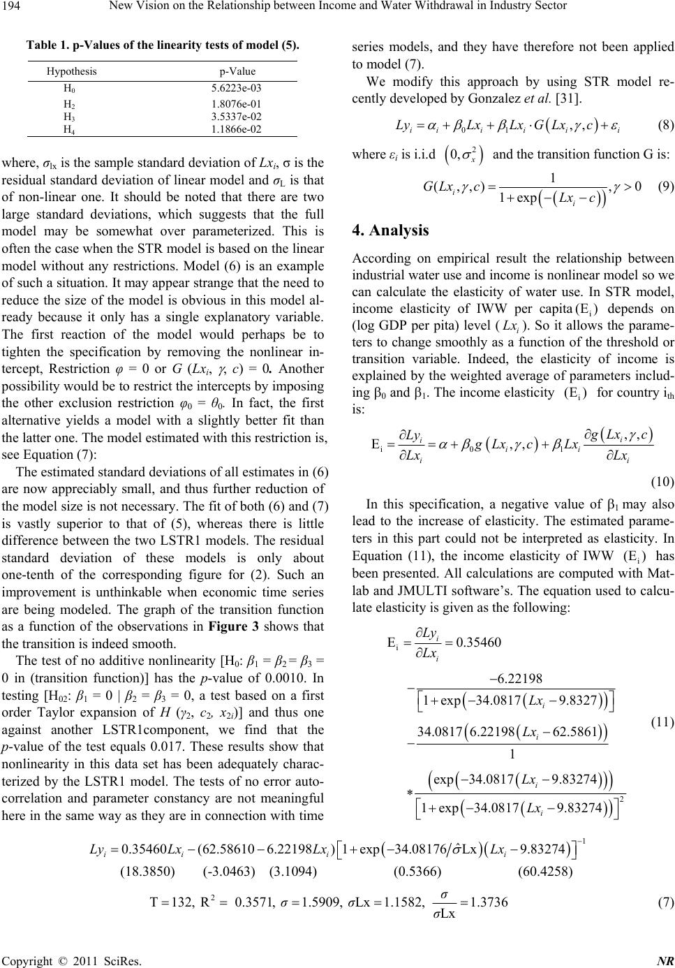 New Vision on the Relationship between Income and Water Withdrawal in Industry Sector 194 Table 1. p-Values of the linearity tests of model (5). Hypothesis p-Value H0 5.6223e-03 H2 1.8076e-01 H3 3.5337e-02 H4 1.1866e-02 where, σlx is the sample standard deviation of Lxi, σ is the residual standard deviation of linear model and σL is that of non-linear one. It should be noted that there are two large standard deviations, which suggests that the full model may be somewhat over parameterized. This is often the case when the STR model is based on the linear model without any restrictions. Model (6) is an example of such a situation. It may appear strange that the need to reduce the size of the model is obvious in this model al- ready because it only has a single explanatory variable. The first reaction of the model would perhaps be to tighten the specification by removing the nonlinear in- tercept, Restriction φ = 0 or G (Lxi, , c) = 0. Another possibility would be to restrict the intercepts by imposing the other exclusion restriction φ0 = θ0. In fact, the first alternative yields a model with a slightly better fit than the latter one. The model estimated with this restriction is, see Equation (7): The estimated standard deviations of all estimates in (6) are now appreciably small, and thus further reduction of the model size is not necessary. The fit of both (6) and (7) is vastly superior to that of (5), whereas there is little difference between the two LSTR1 models. The residual standard deviation of these models is only about one-tenth of the corresponding figure for (2). Such an improvement is unthinkable when economic time series are being modeled. The graph of the transition function as a function of the observations in Figure 3 shows that the transition is indeed smooth. The test of no additive nonlinearity [H0: β1 = β2 = β3 = 0 in (transition function)] has the p-value of 0.0010. In testing [H02: β1 = 0 | β2 = β3 = 0, a test based on a first order Taylor expansion of H (γ2, c2, x2i)] and thus one against another LSTR1component, we find that the p-value of the test equals 0.017. These results show that nonlinearity in this data set has been adequately charac- terized by the LSTR1 model. The tests of no error auto- correlation and parameter constancy are not meaningful here in the same way as they are in connection with time series models, and they have therefore not been applied to model (7). We modify this approach by using STR model re- cently developed by Gonzalez et al. [31]. 01 ,, iiiii LyLxLxG Lxci (8) where εi is i.i.d 2 0, and the transition function G is: 1 (,,), 0 1exp i i GLx cLx c (9) 4. Analysis According on empirical result the relationship between industrial water use and income is nonlinear model so we can calculate the elasticity of water use. In STR model, income elasticity of IWW per capitai depends on (log GDP per pita) level (i). So it allows the parame- ters to change smoothly as a function of the threshold or transition variable. Indeed, the elasticity of income is explained by the weighted average of parameters includ- ing 0 and 1. The income elasticity for country ith is: (E ) i (E ) Lx i01 , E,, , i i ii ii Lx c Ly gLx cLx Lx Lx (10) In this specification, a negative value of 1 may also lead to the increase of elasticity. The estimated parame- ters in this part could not be interpreted as elasticity. In Equation (11), the income elasticity of IWW i has been presented. All calculations are computed with Mat- lab and JMULTI software’s. The equation used to calcu- late elasticity is given as the following: (E ) i 2 E 0.35460 6.22198 1 exp34.08179.8327 34.0817 6.2219862.5861 1 exp 34.08179.83274 1 exp34.08179.83274 i i i i i i Ly Lx Lx Lx Lx Lx (11) 1 ˆ 0.35460(62.586106.22198) 1exp34.08176Lx9.83274 ii ii Ly LxLxLx (18.3850) (-3.0463) (3.1094) (0.5366) (60.4258) 21.5909T, Lx1.1582,1.3132, R 0.3577361, Lx σ σσ σ (7) Copyright © 2011 SciRes. NR 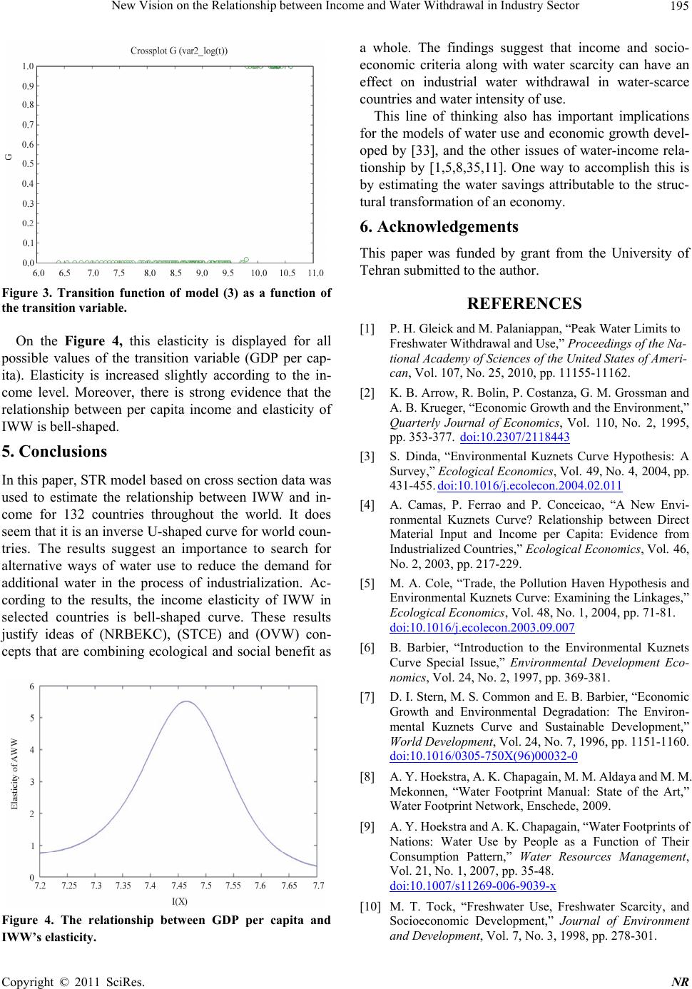 New Vision on the Relationship between Income and Water Withdrawal in Industry Sector 195 Figure 3. Transition function of model (3) as a function of the transition variable. On the Figure 4, this elasticity is displayed for all possible values of the transition variable (GDP per cap- ita). Elasticity is increased slightly according to the in- come level. Moreover, there is strong evidence that the relationship between per capita income and elasticity of IWW is bell-shaped. 5. Conclusions In this paper, STR model based on cross section data was used to estimate the relationship between IWW and in- come for 132 countries throughout the world. It does seem that it is an inverse U-shaped curve for world coun- tries. The results suggest an importance to search for alternative ways of water use to reduce the demand for additional water in the process of industrialization. Ac- cording to the results, the income elasticity of IWW in selected countries is bell-shaped curve. These results justify ideas of (NRBEKC), (STCE) and (OVW) con- cepts that are combining ecological and social benefit as Figure 4. The relationship between GDP per capita and IWW’s elasticity. a whole. The findings suggest that income and socio- economic criteria along with water scarcity can have an effect on industrial water withdrawal in water-scarce countries and water intensity of use. This line of thinking also has important implications for the models of water use and economic growth devel- oped by [33], and the other issues of water-income rela- tionship by [1,5,8,35,11]. One way to accomplish this is by estimating the water savings attributable to the struc- tural transformation of an economy. 6. Acknowledgements This paper was funded by grant from the University of Tehran submitted to the author. REFERENCES [1] P. H. Gleick and M. Palaniappan, “Peak Water Limits to Freshwater Withdrawal and Use,” Proceedings of the Na- tional Academy of Sciences of the United States of Ameri- can, Vol. 107, No. 25, 2010, pp. 11155-11162. [2] K. B. Arrow, R. Bolin, P. Costanza, G. M. Grossman and A. B. Krueger, “Economic Growth and the Environment,” Quarterly Journal of Economics, Vol. 110, No. 2, 1995, pp. 353-377. doi:10.2307/2118443 [3] S. Dinda, “Environmental Kuznets Curve Hypothesis: A Survey,” Ecological Economics, Vol. 49, No. 4, 2004, pp. 431-455. doi:10.1016/j.ecolecon.2004.02.011 [4] A. Camas, P. Ferrao and P. Conceicao, “A New Envi- ronmental Kuznets Curve? Relationship between Direct Material Input and Income per Capita: Evidence from Industrialized Countries,” Ecological Economics, Vol. 46, No. 2, 2003, pp. 217-229. [5] M. A. Cole, “Trade, the Pollution Haven Hypothesis and Environmental Kuznets Curve: Examining the Linkages,” Ecological Economics, Vol. 48, No. 1, 2004, pp. 71-81. doi:10.1016/j.ecolecon.2003.09.007 [6] B. Barbier, “Introduction to the Environmental Kuznets Curve Special Issue,” Environmental Development Eco- nomics, Vol. 24, No. 2, 1997, pp. 369-381. [7] D. I. Stern, M. S. Common and E. B. Barbier, “Economic Growth and Environmental Degradation: The Environ- mental Kuznets Curve and Sustainable Development,” World Development, Vol. 24, No. 7, 1996, pp. 1151-1160. doi:10.1016/0305-750X(96)00032-0 [8] A. Y. Hoekstra, A. K. Chapagain, M. M. Aldaya and M. M. Mekonnen, “Water Footprint Manual: State of the Art,” Water Footprint Network, Enschede, 2009. [9] A. Y. Hoekstra and A. K. Chapagain, “Water Footprints of Nations: Water Use by People as a Function of Their Consumption Pattern,” Water Resources Management, Vol. 21, No. 1, 2007, pp. 35-48. doi:10.1007/s11269-006-9039-x [10] M. T. Tock, “Freshwater Use, Freshwater Scarcity, and Socioeconomic Development,” Journal of Environment and Development, Vol. 7, No. 3, 1998, pp. 278-301. Copyright © 2011 SciRes. NR 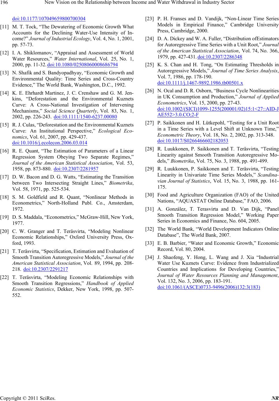 New Vision on the Relationship between Income and Water Withdrawal in Industry Sector Copyright © 2011 SciRes. NR 196 doi:10.1177/107049659800700304 [11] M. T. Tock, “The Dewatering of Economic Growth What Accounts for the Declining Water-Use Intensity of In- come?” Journal of Industrial Ecology, Vol. 4, No. 1, 2001, pp. 57-73. [12] I. A. Shiklomanov, “Appraisal and Assessment of World Water Resources,” Water International, Vol. 25, No. 1, 2000, pp. 11-32. doi:10.1080/02508060008686794 [13] N. Shafik and S. Bandyopadhyay, “Economic Growth and Environmental Quality: Time Series and Cross-Country Evidence,” The World Bank, Washington, D.C., 1992. [14] K. E. Ehrhardt Martinez, J. C. Crenshaw and G. M. Jen- kins, “Deforestation and the Environmental Kuznets Curve: A Cross-National Investigation of Intervening Mechanisms,” Social Science Quarterly, Vol. 83, No. 1, 2002, pp. 226-243. doi:10.1111/1540-6237.00080 [15] R. J. Culas, “Deforestation and the Environmental Kuznets Curve: An Institutional Perspective,” Ecological Eco- nomics, Vol. 61, 2007, pp. 429-437. doi:10.1016/j.ecolecon.2006.03.014 [16] R. E. Quant, “The Estimation of Parameters of a Linear Regression System Obeying Two Separate Regimes,” Journal of the American Statistical Association, Vol. 53, 1958, pp. 873-880. doi:10.2307/2281957 [17] D. W. Bacon and D. G. Watts, “Estimating the Transition between Two Intersecting Straight Lines,” Biometrika, Vol. 58, 1971, pp. 525-534. [18] S. M. Goldfield and R. Quant, “Nonlinear Methods in Econometrics,” North-Holland Publ. Co., Amsterdam, 1972. [19] D. S. Maddala, “Econometrics,” McGraw-Hill, New York, 1977. [20] C. W. Granger and T. Teräsvirta, “Modeling Nonlinear Economic Relationships,” Oxford University Press, Ox- ford, 1993. [21] T. Teräsvirta, “Specification, Estimation and Evaluation of Smooth Transition Autoregressive Models,” Journal of the American Statistical Association, Vol. 89, 1994, pp. 208- 218. doi:10.2307/2291217 [22] T. Teräsvirta, “Modeling Economic Relationships with Smooth Transition Regressions,” Handbook of Applied Economic Statistics, Dekker, New York, 1998, pp. 507- 552. [23] P. H. Franses and D. Vandijk, “Non-Linear Time Series Models in Empirical Finance,” Cambridge University Press, Cambridge, 2000. [24] D. A. Dickey and W. A. Fuller, “Distribution ofEstimators for Autoregressive Time Series with a Unit Root,” Journal of the American Statistical Association, Vol. 74, No. 366, 1979, pp. 427-431. doi:10.2307/2286348 [25] K. S. Chan and H. Tong, “On Estimating Thresholds in Autoregressive Models,” Journal of Time Series Analysis, Vol. 7, 1986, pp. 178-190. doi:10.1111/j.1467-9892.1986.tb00501.x [26] N. Ocal and D. R. Osborn, “Business Cycle Nonlinearities in UK Consumption and Production,” Journal of Applied Econometrics, Vol. 15, 2000, pp. 27-43. doi:10.1002/(SICI)1099-1255(200001/02)15:1<27::AID-J AE552>3.0.CO;2-F [27] P. Saikkonen and H. Lütkepohl, “Testing for a Unit Root in a Time Series with a Level Shift at Unknown Time,” Econometric Theory, Vol. 18, No. 2, 2002, pp. 313-348. doi:10.1017/S0266466602182053 [28] R. Luukkonen, P. Saikkonen and T. Teräsvirta, “Testing Linearity against Smooth Transition Autoregressive Mo- dels,” Biometrika, Vol. 75, No. 3, 1988, pp. 491-499. [29] R. Luukkonen, P. Saikkonen and T. Teräsvirta, “Testing Linearity in Univariate Time Series Models,” Scandina- vian Journal of Statistics, Vol. 15, No. 3, 1988, pp. 161- 175. [30] Food and Agriculture Organization (FAO) of the United Nations, “AQUASTAT Online Database,” FAO, 2006. [31] A. González, T. Terasvirta and D. Van Dijk, “Panel Smooth Transition Regression Model,” Working Paper Series in Economics and Finance, No. 604, 2005. [32] The World Bank, “World Development Indicators Online Database”, The World Bank, 2007. [33] E. B. Barbier, “Water and Economic Growth,” Economic Record, Vol. 80, 2004. [34] J. Shaofeng, Y. Hong, L. Wang and J. Xia “Industrial Water Use Kuznets Curve: Evidence from Industrialized Countries and Implications for Developing Countries,” Journal of Water Resources Planning and Management, Vol. 132, No. 3, 2006, pp. 183-191. doi:10.1061/(ASCE)0733-9496(2006)132:3(183)
|