Energy and Power Engineering
Vol.09 No.04(2017), Article ID:75242,14 pages
10.4236/epe.2017.94B016
Research on Multi-Scale Modeling of Grid-Connected Distributed Photovoltaic Power Generation
Chen Lv1,2, Wanxing Sheng1, Keyan Liu1, Xinzhou Dong2
1China Electric Power Research Institute, Haidian District, Beijing, China
2Department of Electrical Engineering, Tsinghua University, Beijing, China


Received: March 2, 2017; Accepted: March 30, 2017; Published: April 6, 2017
ABSTRACT
The complexity of distribution network model mainly depends on the model scale of grid-connected distributed photovoltaic (PV) power generation. Therefore, the simulation performance of multi-scale PV model is the key factor of the simulation accuracy in the specific operating scenarios of distribution network. In this paper, a multi-scale model of grid connected PV distributed generation system is proposed based on the mathematical model of grid- connected distributed PV power generation. It is analyzed that differences of simulation performance, such as adaptability of simulation step size, accuracy of output and the effect on voltage profile of distribution network, between PV models with different scales in IEEE 33 node example. Simulation results indicate that the multi-scale model is effective in improving the accuracy and efficiency of simulation under different operating conditions of distribution network.
Keywords:
PV, Distributed Generation, Multi-Scale Modeling, Simulation Step Size, Output Power, Voltage Profile

1. Introduction
Distributed photovoltaic (PV) grid-connected power generation is an important application of solar energy, which can replace fossil fuels and reduce environmental pollution [1] [2]. Therefore, it is significant for the study of distribution network that build an appropriate model of distributed PV grid-connected power generation.
Researchers have built a number of PV models with different scales. A mathematical model of the PV arrays is established [3], which is able to simulate the output characteristics of photo-voltaic arrays under both normal and partial occlusion circumstances. The maximum power point tracking (MPPT) technique of PV arrays is improved to adapt to partial occlusion [4]. Short term prediction output power of PV arrays is realized with the detailed mathematical model of the PV arrays [5]. A detailed dynamic model of PV power generation system including PV array, inverter, controller and grid is established by Huang [6]. Using the method of eigenvalue analysis, Li analyzes the stability of the PV detailed dynamic model subjected to various external disturbances [7]. a detailed model of grid-connected PV inverter is built in [8] [9] [10], which forms a multi-mode control strategy based on the existing inverter control strategy, including reactive power compensation and active power control. A parallel-connected multi-inverter model is established to analyze its fundamental resonance characteristics [11]. Using this model, it is concluded that the resonance of PV inverter is directly related to the inverter control and carrier synchronization.
Although a variety of PV models have been established, the scope of application of each model is limited by its model scale. In this paper, a multi-scale model of grid-connected distributed PV power generation will be established. Through the analysis of the simulation performance of the multi-scale model, PV modeling scale under different application conditions will be specified and the simulation accuracy and efficiency of distribution network can be improved.
2. Mathematical Model of PV Generation
2.1. Composition of PV Generation System
As shown in Figure 1, the overall structure of PV generation system includes two main components: the DC side and AC side. The DC side of the PV model is mainly composed of several modules, such as PV array, DC converter and MPPT. The AC side of the PV model consists of several modules, such as inverters, filters and inverter control modules. The solar energy is transformed into direct current by the PV panels, boosted by the DC side and MPPT, then trans-

Figure 1. Schematic diagram of PV generation system.
formed into alternating current by the inverter and filtering process, finally sent to the grid as three-phase alternating current. In this section, the mathematical models of the components of the PV power generation system will be established.
2.2. Mathematical Model of the DC Side
2.2.1. PV Arrays
A PV cell is a device that converts solar energy into electrical energy. A PV array consists of a large number of PV cells to produce large amounts of electrical energy. The equivalent circuit of the PV array is shown in Figure 2, where Iph represents the photo generated current, Id represents the diode junction current, Rs represents the series resistance, and Rsh represents the parallel resistance.
According to the principle of the circuit, the relationship between the output current and the output voltage of the PV array is shown in Equation (1), where I0 represents the reverse saturation current, q represents the electronic charge, n represents the diode factor, k represents the Boltzmann constant, and T re- presents the absolute temperature.
 (1)
(1)
Equation (1) can be simplified using four measurable parameters such as open circuit voltage Voc, short circuit current Isc, maximum power point voltage Vm, and maximum power point current Im. The simplified expression is as Equations (2)-(4).
 (2)
(2)
 (3)
(3)
 (4)
(4)
The PV array mathematical model consists of Equations (2) to (4). The model can directly reflect the influence of external environment on the output characteristics of PV arrays, because its four parameters (Voc, Isc, Vm, Im) change directly

Figure 2. Equivalent circuit of PV Arrays.
with the light intensity S and ambient temperature T.
2.2.2. DC-DC Converter
In this paper, Boost circuit is chosen as the DC-DC converter of PV power generation unit. Its topology is shown in Figure 3. When the switch Tc is conducting, the input voltage will charge the inductor L, in order to make its current rise. When Tc is turned off, L starts to discharge. Then its voltage and input voltage are superimposed on each other, so that the output voltage is higher than the input voltage.
According to the principle of Boost circuit, its input resistance can be expressed as follows:
 (5)
(5)
As shown in Equation (5), when the load resistance R is fixed, the greater the switch duty cycle D, the smaller the input impedance Rin, and vice versa.
2.2.3. MPPT Strategy
As shown in the analysis above, Rin can be changed by adjusting D. Therefore, the MPPT can be implemented by controlling the input resistance to be equal to the PV output resistance. In this paper, the perturbation observation method is adopted as the MPPT strategy, and the algorithm flow is shown in Figure 4.

Figure 3. Schematic diagram of boost circuit.

Figure 4. Flowchart of perturbation observation.
2.3. Mathematical Model of the AC Side
2.3.1. DC-AC Converter
In this paper, the DC-AC converter converter is composed of a three-phase full-bridge inverter and an LC-type filter. The topology of the converter is shown in Figure 5.
The state equation of the DC-AC converter in the three-phase stationary coordinate system can be obtained based on the Kirchhoff voltage law (KVL).
 (6)
(6)
In order to facilitate the control, the three-phase static coordinate system is transformed into two-phase dq rotating coordinate system through the park transformation. The equation of state of the DC-AC converter in rotating coordinate system is as follows:
 (7)
(7)
At the same time, the power calculation formula in the rotating coordinate system can be derived:
 (8)
(8)
If the gridside voltage space vector direction and d-axis direction is the same, eq is zero when the network side voltage is a standard symmetrical three-phase sine wave. Therefore, Equation (8) can be simplified as follows:
 (9)
(9)
The control strategy of DC-AC converter can be designed by using the ma-

Figure 5. Topology of DC-AC converter.
thematical relations of Equation (7) and Equation (9).
2.3.2. Inverter Control Strategy
Inverter control strategy includes two types: voltage source control strategy and current source control strategy. The current-source control strategy is used in this paper to control the inverter of grid-connected PV models.
In this control strategy (Figure 6), firstly, the power reference value ,
,  is transformed into the current reference value
 ,
,  by using Equation (9). Then, the inverter output voltage reference value
 ,
,  is obtained through the current control loop. Finally, the decoupling control of the inverter output power is realized by controlling the duty cycle of each power electronic switch in the inverter with the voltage reference.
3. Multi-Scale Modeling of PV
3.1. PV Model Classification by Scale
In the different application scenarios, the mathematical model of the PV power generation system described above can be transformed into dynamic models of different scales. According to the scale of the model, dynamic model can be divided into three types: Generalized load model, Model with DC voltage source, and Detailed model.
3.2. Generalized Load Model
During the steady state analysis of the power system, the internal structure, the interaction between the various components and the specific adjustment process of internal parameters of PV power generation system can be ignored. Only the average active output power P and the average reactive power output Q over a period of time are used to modify the load data in the power flow calculation equation to simulate the influence of the PV power generation system on the power grid. In this case, the PV power generation system is regarded as a generalized load with negative power consumption (−P, −Q) (Figure 7).
3.3. Model with DC Voltage Source
The DC-side output voltage can be assumed to be constant if the light intensity

Figure 6. Current-source control strategy diagram.
and temperature are constant, or if the PV system is equipped with a large capacity energy storage device. In this case, the DC-side model structure can be simulated only with a DC voltage source within a certain output power range. The AC side consists of detailed models of the power electronic switch, the LC filter and the control module, simulating the dynamic switching process of the power electronic switch inside the inverter (Figure 8).
3.4. Detailed Model
When considering the effects of light intensity, temperature variation, MPPT and DC bus voltage variation on the output of PV power generation system, further refinement of the model scale on the DC side of the PV power generation system should be made. The DC side of the PV system consists of detailed models of PV panels, DC-DC converters, and MPPT. It simulates the dynamic output characteristics of the PV system with the AC side detail model (Figure 9).

Figure 7. Generalized load model.

Figure 8. PV system model with DC voltage source.

Figure 9. Detailed model of PV system.
4. Analysis of Simulation Performance of Mul-Ti-Scale PV Model
4.1. Application Scenario
In order to compare the simulation performance of the multi-scale PV models, IEEE33 node is chosen as the PV application scenario in this paper. As shown in Figure 10, the PV model is connected to the MV distribution network through a transformer, and the access point is the end node of the longest feeder in the example (node 17). The rated voltage of the PV model is 380 V, the rated output active power is 50 kW, and the rated reactive power is 0.
Based on the above application scenarios, the simulation performance of PV models with different scales is compared in this paper. Simulation hardware environment is a personal computer which has installed MATLAB 2011b, 3 GHz CPU, and 2 GB memory. The simulation model is shown in Figure 11.
The simulation performance of the model mainly includes the dynamic characteristic and the steady state characteristic. Dynamic characteristics are embodied in two aspects: simulation speed and simulation precision. On the premise of ensuring the convergence of the calculation process, the larger simulation step size, and the faster simulation speed. The simulation precision is reflected in the simulation accuracy of the output power of the PV model, when the light intensity changes. In addition, the main factor is the influence of the PV model on the distribution network voltage profile, when the output power is constant.
Therefore, this paper makes a comparison of the performance of the multi-scale PV model in the step size adaptability, output power accuracy, and the effect on distribution network voltage profile.

Figure 10. Topology of PV application scenarios.
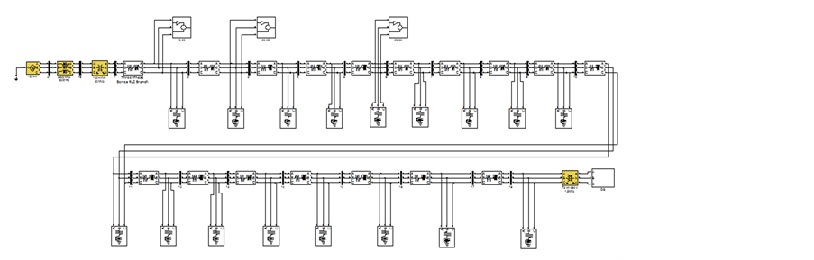
Figure 11. Multi-scale simulation model of grid-connected PV power generation system.
4.2. Simulation Result
4.2.1. Step Size Adaptability of Models
In order to compare the step size adaptation of different scale models, the different scales of the PV model are calculated in the application scenarios, with three different simulation steps: 5 μs, 50 μs and 200 μs. The output currents of the PV models are recorded.
As shown in Figure 12, when the step size is 5 μs, the output current of all three models can reach the stable state within the 0.04 s. Thus, in the case of 5 step size, the three models are all able to effectively simulate the output characteristics of the PV model in the dynamic state.
As shown in Figure 13, when the step size is increased to 50 μs, the model with DC voltage source and the generalized load model are still able to maintain stable output currents, but the output current of detailed model produces fluctuation with about 20 times the rated amplitude. Due to the fluctuations in the 0.2 seconds is still not able to decay to the rated value, the output current waveform can be considered a serious distortion. It shows that the simulation capability of the detailed model is more sensitive to the simulation step than two other models. At present, the step size needed by the distribution network digital analog

Figure 12. Output currents (Ts = 5 μs).

Figure 13. Output currents (Ts = 50 μs).
hybrid real-time simulation is about 20 μs - 50 μs. Thus, the PV detailed model is not completely applicable to the distribution network digital analog hybrid real- time simulation.
Since the detailed model has a large fluctuation when the simulation step size is 50 μs, only the output current waveforms of the model with DC voltage source and the generalized load model are compared when the simulation step size is 200 μs.
As shown in Figure 14, when the simulation step size is increased to 200 μs, the amplitude and period of DC voltage source model output current are basically the same as the generalized load model, although the local waveform of its output current fluctuates. It can be seen that the model with DC voltage source and the generalized load model can accurately represent the output characteristics of PV generation systems even in the step size of 200 μs.
In addition, although the model with DC voltage source and the generalized load model have the same excellent step adaptability, the model with DC voltage source has a higher application value, considering its ability to simulate complex dynamic characteristics.
4.2.2. Output Power Accuracy of Models
In order to compare the output power of the multi-scale PV models under the same conditions, the simulation step is set as 5 μs and the light intensity is changed step by step according to the order of 100%, 30% and 70% of the rated value. The output active power curves of the three models are plotted in the same figure (Figure 15) while the output power of the PV array is indicated by a dotted line as a reference.
It can be seen from Figure 15 that the active power output of the three PV models can be stabilized within 0.1 second after each illumination intensity change, and the variation law of the output curve is the same as the light intensity. It indicates that all three PV models have a certain ability to simulate the PV output power within a certain range.
The local curves of the output power of the PV models at different light intensities are shown in Figure 16. It can be seen from Figure 16(a) that the output

Figure 14. Output currents (Ts = 200 μs).

Figure 15. Output active power of models.
power of three PV models is approximately equal to the output power reference value under the rated light intensity. When the light intensity changes, as shown in Figure 16(b) and Figure 16(c), PV detailed model can accurately simulate the output power of PV arrays. On the contrary, the other two models do not have DC side detailed structure, only adjust the output power with the change ratio of light intensity, resulting in a certain error in output power. Therefore, when the needed accuracy of PV output power is high, it is appropriate to select the PV detailed model to simulate the PV generation system.
4.2.3. Effect of Models on Distribution Network Voltage Profile
In order to compare the influence of PV models on voltage profile in distribution network, the voltage profile curves of the three PV models under stable operation are plotted on the same figure (Figure 17). At the same time, the voltage profile of the distribution network without PV is indicated by a red dotted line.
It can be seen that when the PV model is connected to the distribution network, the voltage of each point has a different degree of rise, and the three PV models have no significant difference in the voltage profile. Therefore, when only the voltage profile is the object of study, the generalized load model with higher computation speed is more suitable.
5. Conclusions
A multi-scale model of grid-connected PV power generation system is built in this paper. The following conclusions can be drawn by comparing the performance of different scale PV models in simulation step adaptability, output power accuracy and the effect on voltage profile of distribution network.
1) The model with DC voltage source and the generalized load model have better step adaptability than the detail model of PV generation system. The model with DC voltage source has a higher application value, considering its ability to simulate complex dynamic characteristics.
2) When the needed accuracy of PV output power is high, it is appropriate to select the PV detailed model to simulate the PV generation system.
 (a)
(a)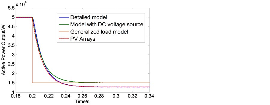 (b)
(b) (c)
(c)
Figure 16. (a) Segmented output curve; (b) Segmented output curve; (c) Segmented output curve.
3) The three scales of PV models have no significant difference in the voltage profile. Therefore, when only the voltage profile is the object of study, the generalized load model with higher computation speed is more suitable.

Figure 17. Distribution network voltage profile curve.
Acknowledgements
This paper is supported by Research Program of State Grid Corporation in China (PD71-15-042) and Research Program of State Grid Corporation in Ningxia (PDB11201601764).
Cite this paper
Lv, C., Sheng, W.X., Liu, K.Y. and Dong, X.Z. (2017) Research on Multi-Scale Modeling of Grid- Connected Distributed Photovoltaic Power Generation. Energy and Power Engineering, 9, 127-140. https://doi.org/10.4236/epe.2017.94B016
References
- 1. Liu, S.C., Liu, P.X.P. and Wang, X.Y. (2016) Stability Analysis of Grid-Interfacing Inverter Control in Distribution Systems With Multiple Photovoltaic-Based Distributed Generators. IEEE Transactions on Industrial Electronics, 63, 7339-7348. https://doi.org/10.1109/TIE.2016.2592864
- 2. Zhang, X., Cao, R.X., etc. (2010) Solar PV grid-connected power generation and inverter control. Mechanical Industry Press, Beijing, 9.
- 3. Rahman, S.A., Varma, R.K. and Vanderheide, T. (2014) Generalised Model of a photovoltaic panel. IET Renewable Power Generation, 8, 217-229. https://doi.org/10.1049/iet-rpg.2013.0094
- 4. Ghasemi, M.A., Forushani, H.M. and Parniani, M. (2016) Partial Shading Detection and Smooth Maximum Power Point Tracking of PV Arrays Under PSC. IEEE Transactions on Power Electronics, 31, 6281-6292. https://doi.org/10.1109/TPEL.2015.2504515
- 5. Radvansky, M., Kudělka, M. and Snásel, V. (2014) Short Term Power Prediction Of The Photovoltaic Power Station Based on Comparison of Power Profile Sequences Using F-Score Computation. IEEE International Conference on Systems, Man, and Cybernetics, 3497-3502.
- 6. Huang, H.Q., Mao, C.X., Lu, J.M., et al. (2012) Small Signal Modeling and Analysis of PV Power Generation System. Proceeding of the CSEE, 22, 7-14+24.
- 7. Li, N.Y., Liang, J. and Zhao, Y.S. (2011) Study on dynamic modeling and stability of grid-connected PV power station. Proceeding of the CSEE, 10, 12-18.
- 8. Mishra, S., Ramasubramanian, D. and Sekhar, P. C. (2013) A Seamless Control Methodology for a Grid Connected and Isolated PV-Diesel Microgrid. IEEE Transactions on Power Systems, 28, 4393-4404. https://doi.org/10.1109/TPWRS.2013.2261098
- 9. Zhang, H. and Xie, K.G. (2014) Simulation and Analysis of PV Power Station Based on PSCAD. Power System Technology, 7, 1848-1852.
- 10. Baumann, K., Strache, S., Wunderlich, R., et al. (2013) Concept Study for Fully Integrated and Photovoltaic Inverter. Annual Conference of the IEEE Industrial Electronics Society, 6974-6979.
- 11. Zhang, X., Yu, C.Z., Liu, F., et al. (2014) Parallel Modeling and Resonant Analysis of PV Multi-Inverters. Proceeding of the CSEE, 3, 336-345.