Journal of Service Science and Management, 2011, 4, 280-283
doi:10.4236/jssm.2011.43033 Published Online September 2011 (http://www.SciRP.org/journal/jssm)
East Asia n Econ omic Growt h—An Evolutionary
Perspecti ve
Fariba Hashemi
Swiss Federal Institute of Technology, Lausanne, Switzerland.
Received June 27th, 2011; revised August 2nd, 2011; accepted August 18th, 2011.
ABSTRACT
The High Performing Asian Economies have been the fastest growing economies anywhe re, anytime. This phenomenal
growth experience has stimulated extensive research on its determinants. What is less known however, is dynamics of
the distribution of income. This paper considers a statistical model to describe convergence of cross-country incomes
acro ss the High Performing Asian Economies. The empirical results illustrate th at diffusio n is a p otential te chnique for
the analysis of spatial dynamics of economic growth.
Keywords: East Asian Economic Growth, Evolutionary Perspective
1. Introduction
The High-Performing Asian Economies (HPAE) have
been the fastest growing economies anywhere, anytime1.
Figure 1 and Table 1 illustrate the strong economic
growth which spread like a wave over the region between
the years of 1960-1995.
Compared to large parts of Asia, Africa and Latin
America, the High Performing Asian Economies have
bee n unu suall y s uc ce ss f ul a t a c hie vi n g high gr owth ra tes.
Figure 1. Str o ng economic growth spread like a wave over
Asia.
Table 1. A sia n economic growth.
(Avera ge Real GDP P erc ent P er Annum)
1960-1969 1970-1979 1980-1989 1990-1995
East Asia
Japan 10.5 5.2 3.8 1.9
Asian “Tigers”
Hong Kong - 7.9 3.0 5.1
Korea 7.7 9.4 8.1 7.9
Taiwan 9.8 10.2 8.1 6 .4
Singapore - 9.5 7.4 8.6
Other high growth*
Malaysis - 8.1 5.8 8.9
Thailand 8.3 7.4 7 .3 8.9
Indonesia 4.0 7.8 5.8 7.1
Other East Asian
Chian 2.9 7.5 9.4 10.2
Philippines 4.9 6.1 2.0 2.4
Vietnam - - - 7.7
Other Asian
India 3.7 3.2 6 .0 4.8
Source: UBS Publi cations 1996, reproduced with permission .
At the same time that the HPAE were growing at over
5.5%, richer industrial economies were growing at
around 2%, South Asia likewise at 2%, and Latin Amer-
ica at 1%. Africa and the Middle East were shrinking2.
The phenomenal growth in HPAE altered the global
economic balance and contributed to closing of the eco-
1For purposes of this paper, High Performing Asian Econo
mies in c lud e:
China, Hong Kong, Indonesia, Japan, Malaysia, South Korea, Singa-
pore, Taiwan, and Thailand.

East Asian Economic Growth—An Evolutionary Perspective
281
nomic gap between the OECD and developing countries.
The growth experience of East Asia has stimulated
extensive research on its determinants [1-5]. Much a tten-
tion has been devoted to the explanation of the shape of
the distribution of income in the region by reference to
steady state arguments. What is less known however, is
the dynamics in question. To fill this gap, the present
paper examines the dynamics in the cross-sectional dis-
tribution of income in High Performing Asian Econo-
mies.
2. The Model
Consider a region consisting of countries with different
levels of income. The set of country incomes forms a
long-run distribution which evolves over time. Assume
that t he d ynamics o f thi s dist rib ution re ly on t wo co unte-
racting forces: 1) a mean-reversion process along time,
driven by mobility of factors of production [6]; and 2) a
diffusion process across regions, driven by search and
learning [7-9].
Consistent with the above, assuming that income be-
haves like a stochastic process and that it is continuous
and Markovian, the evolution over time of income dis-
tribution can be expressed by the following classical
second order partial differential equation:
( ) ( )
2
2
ff
u sf
ts s
λε
∂∂ ∂
+ −=
∂∂ ∂
(1)
where f measures probability density and s measures in-
come. λ represents the income adjustment rate, u repre-
sents the mean of the distribution in the long run, and ε
represents a diffusion parameter3.
3. Empirical application
3.1. Data and Descriptive Statistics
The empirical analysis employs data on Gross Domestic
Product (GDP) per capita of High Performing Asian
Economies from 1980 to 2007. Figure 2 illustrates the
evolution of the distribution of GDP per capita for the
population4. A steady growth can be observed, with the
South East Asian financial crisis standing out. Table 2
shows the descriptive of GDP per capita for N = 28 years
of data.
3.2. Estimation
The model has been applied to log GDP per capita dis-
tribution of the HPAE as a function of time, to estimate
the five model parameters5. u0 and u denote the initial
and long-run mean of the distribution respectively. σ0
represents the initial standard deviation,
ε
represents
the diffusion parameter, and λ represents the income ad-
justment rate. Table 3 reports estimates for the five
model parameters.
The value for the income adjustment parameter
λ
is
Table 2. Descriptive of GDP per capita for HPAE from
1980 to 200 7.
N Minimum Maximum Mea n Std . Deviation
GDP 28 3624.87 22790.29 11317. 03 5473.38
Figure 2. Evolution of GDP.
2These fi g u res a re a n n u a l a vera ges , based on GDP per person, 1965-1996.
The author acknowledges and thanks Minimax consulting for the statistical
analysis in this paper.
3Ref [10] provi des a full analysis of this mod el but in a different cont ext.
4Data graphed a re yearly mea ns.

East Asian Economic Growth—An Evolutionary Perspective
282
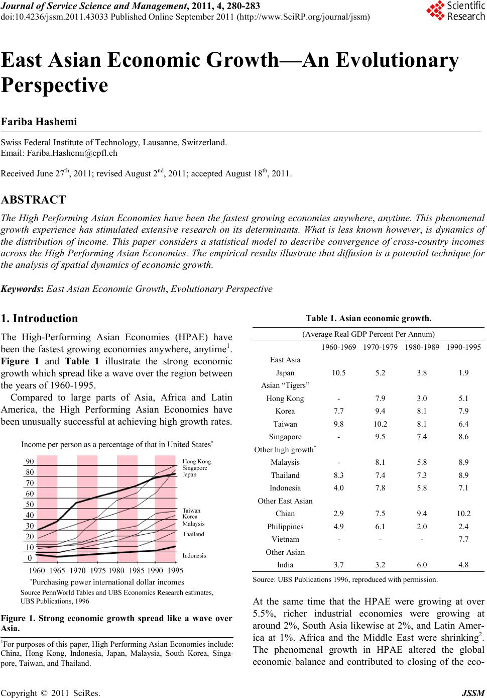
Table 3. P arameter estimates.
Paramet er Valu e Std Error t-Value
λ 1.88 1.01 0.31
u 1.57 0.02 32.54
u0 1.37 0.02 13.15
σ 1.06 0.03 10.90
ε 0.58 0.03 9.90
positive as expected. The va lue for the dif fusio n par ame-
ter
ε
is small and positive, likewise conforming to our
theoretical predictions. The results predict that if one
begins with a normal distribution and allows the model
drive the distribution, the distribution variance will tend
toward a c ons tant
2
lim
t
t
σ ελ
→∞
=
, and concentrated around
a mean
u
. Moreover, it can be observed that the mean
and variance of the distribution is clearly evolving, cor-
responding to our theoretical predictions.
4. Conclusions
Our findings have interesting implications for dynamics
of the distribution of income across the High Performing
Asian Economies. The results suggest that diffusion is a
potential technique for the analysis of spatial dynamics
of ec onomic growth.
REFERENCES
[1] T. Ito and A. Krueger, “Growth Theories in Light of the
East Asian Experience,” University of Chicago Press,
Chi c a go, 1995.
[2] J. Braude and Y. Menashe, “The Asian Miracle: Was it a
Capital-Inten sive Struct ural Change?” Journal of Interna-
tional Trade and Economic Development, Vol. 20, No. 1 ,
2011, pp . 31-51. doi:10.1080/09638199.2011.538183
[3] A. Charles, G. Fontana and A. Srivastava, “India, China
and the East Asian Miracle,” Cambridge Journal of Re-
gions, Economy and Society, Vol. 4, No. 1, 2011, pp.
29-48.
[4] H. Leung, “Two New Lessons from the Asian Miracles,”
Journal of the Asia Pacific Economy, Vol. 12, No. 1,
2007, pp . 1-16. doi:10.1080/13547860601083488
[5] J. Kruger, U. Cantner an d H. Hanusch, “Total Factor
Productivity, the East Asian Miracle, and the World Pro-
duction Frontier,” Review of World Econo mics, Vol. 136,
No. 1, 2000, pp. 111-36.
[6] R. Lu cas, “Trade and t he Diffusion of the Industrial Rev-
olution,” American Economic Journal: Macroeconomics,
Vol. 1, No. 1, 2009, pp. 1-25.
[7] D. Levine, “Neuroeconomics?” International Review of
Economics, 2011 f ort hc oming .
[8] J. Hirshleifer, “Evolutionary Models in Economics and
La w: Cooperation versus Conflict Strategies,” Economic
Approaches to Law Series, Vol. 3, 2007, pp. 189-248.
[9] B. McKelvey, “Toward a 0th Law of Thermodynamics:
Order-Creation Complexity Dynamics from Physics and
Biology to Bioeconomics,” Journal of Bioeconomics, Vol .
6, No. 1, 2004, pp. 65-96.
doi:10.1023/B:JBIO.0000017280.86382.a0
[10] F. Hashemi, “A Dynamic Model of Size Distribution of
Firms Applied to US Biotechnology and Trucking Indus-
tries,” Small Business Economics, Vol. 21, No. 1, 2002,
pp. 1-10.
[11] M.-O. Hongler, R. Filliger and P. Blanchard, “Soluble
Models for Dynamics Driven by a Super-Diffusive Noi-
se,” Ph ysica A: Statistical Mechanics and Its App lications,
Vol. 370, No. 2, 2006, pp. 301-315.
doi:10.1016/j.physa.2006.02.036
[12] M.-O. Hongler, H. Soner and L. Streit, L, “Stochastic
Control for a class of Random Evolution Models,” Ap-
plied Mathematics and Optimization, Vol. 49, No. 2,
2004, pp . 113-121.
[13] O. Besson and G. de Montmollin, “Space-Time Integra-
ted Least Squares: A Time-Mar ching Approach,” Inter-
national Journal for Numerical Methods in Fluids, Vol.
44, No. 5, 2004, pp. 525-543. doi:10.1002/fld.655
[14] F. Hashemi, “An Evolutionary Model of the Size Distri-
bution of Firms,” Journal of Evolutionary Economics,
Vol. 10, No. 5, 2000, pp. 507-521.
doi:10.1007/s001910000048
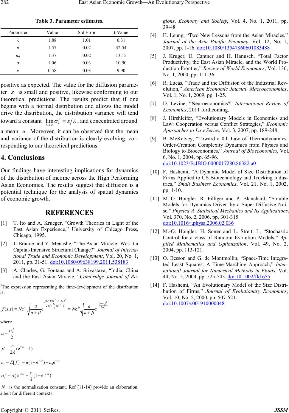
5The expression representing the time-
development of the distribution
is:
2
02
22 2
0
(( )e)()
2
2(e 1)2
(,)=e e=e e
t
t
t
t
su uusu
tt
aa
f stNN
aa
λ
λ
ε
σσ
λλ
λ
ββ
− +−
−−
−
+−
++
where
2
0
=2 a
σ
2
= (e1)
2
t λ
ε
βλ
−
0
=[] =(1e)e
tt
tt
u Efuu
λλ −−
−+
2 222
0
=e(1 e)
tt
t
λλ
ε
σσ λ
−−
+−
N
is the normalization constant. Ref [11-
14] provide an elaboration,
albeit for different contexts.