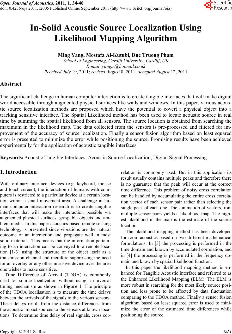Open Journal of Acoust i c s , 2011, 1, 34-40
doi:10.4236/oja.2011.12005 Published Online September 2011 (http://www.SciRP.org/journal/oja)
In-Solid Acoustic Source Localization Using
Likelihood Mapping Algorithm
Ming Yang, Mostafa Al-Kutubi, Duc Truong Pham
School of Engineering, Cardiff University, Cardiff, UK
Received July 19, 201 1; revised August 8, 2011; accepted August 12, 2011
Abstract
The significant challenge in human computer interaction is to create tangible interfaces that will make digital
world accessible through augmented physical surfaces like walls and windows. In this paper, various acous-
tic source localization methods are proposed which have the potential to covert a physical object into a
tracking sensitive interface. The Spatial Likelihood method has been used to locate acoustic source in real
time by summing the spatial likelihood from all sensors. The source location is obtained from searching the
maximum in the likelihood map. The data collected from the sensors is pre-processed and filtered for im-
provement of the accuracy of source localization. Finally a sensor fusion algorithm based on least squared
error is presented to minimize the error while positioning the source. Promising results have been achieved
experimentally for the application of acoustic tangible interfaces.
Keywords: Acoustic Tangible Interfaces, Acoustic Source Localization, Digital Signal Processing
1. Introduction
With ordinary interface devices (e.g. keyboard, mouse
and touch screen), the interaction of humans with com-
puters is restricted to a particular device at a certain loca-
tion within a small movement area. A challenge in hu-
man computer interaction research is to create tangible
interfaces that will make the interaction possible via
augmented physical surfaces, graspable objects and am-
bient media. In this paper acoustics-based remote sensing
technology is presented since vibrations are the natural
outcome of an interaction and propagate well in most
solid materials. This means that the information pertain-
ing to an interaction can be conveyed to a remote loca-
tion [1-3] using the structure of the object itself as a
transmission channel and therefore suppressing the need
for an overlay or any other intrusive device over the area
one wishes to make sensitive.
Time Difference of Arrival (TDOA) is commonly
used for source localization without using a universal
timing mechanism as shown in Figure 1. The principle
of the TDOA localisation is to measure the time delays
between the arrivals of the signals to the various sensors.
These delays result from the distance differences from
the acoustic impact sources to the sensors at known loca-
tions. To determine time delay of real signals, cross cor-
relation is commonly used. But in this application its
result usually contains multiple p eaks and therefore there
is no guarantee that the peak will occur at the correct
time difference. This problem of noisy cross correlation
can be handled by accumulating the entire cross correla-
tion vector of each sensor pair rather than selecting the
single peak of each one. The summation of vectors from
multiple sensor pairs yields a likelihood map. The high-
est likelihood in the map is the estimate of the source
location.
The likelihood mapping method has been developed
for room acoustics based on two different mathematical
formulations. In [3] the processing is performed in the
time domain and known by accumulated correlation, and
in [4] the processing is performed in the frequency do-
main and known by sp atial likelihood function.
In this paper the likelihood mapping method is en-
hanced for Tangible Acoustic Interface and referred to as
the Enhanced Likelihood Mapping (ELM). The ELM is
more robust in searching for the most likely source posi-
tion and less prone to be affected by data fluctuation
comparing to the TDOA method. Finally a sensor fusion
algorithm based on least squared error is used to mini-
mize the error of the estimated time differences while
positioning the source.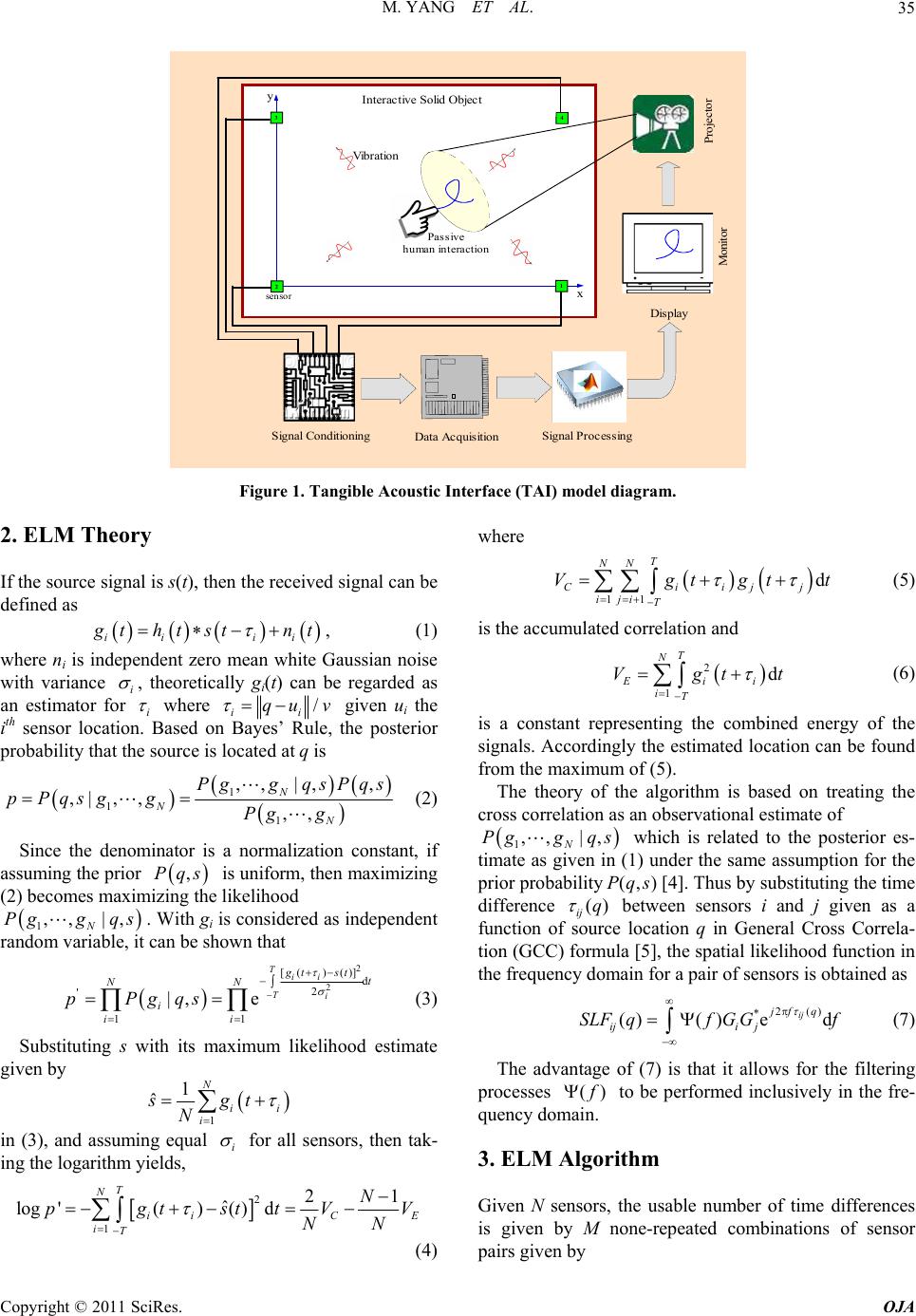

M. YANG ET AL. 35
4
sensor
1
3
2
x
y
Passive
human inte raction
Signal ConditioningD ata Acqu isitionSignal Proc es s ing
Display
Monit or
Projector
Int era ctive So lid O bject
Vibrati on
Figure 1. Tangible Acoustic Interface (TAI) model diagram.
2. ELM Theory
If the source signal is s(t), then the received signal can be
defined as
   
ii ii
g
thtst nt  , (1)
where ni is independent zero mean white Gaussian noise
with variance i

, theoretically gi(t) can be regarded as
an estimator for i

where /
ii
qu v   given ui the
ith sensor location. Based on Bayes’ Rule, the posterior
probability that the sou rce is located at q is

 

1
11
,, |,,
,|, ,,,
N
NN
Pgg qsPqs
pPqsg gPg g 


 (2)
Since the denominator is a normalization constant, if
assuming the prior

,Pqs is uniform, then maximizing
(2) becomes maximizing the likelihood

1,, |, N
Pgg qs. With gi is considered as independ ent
random variable, it can be shown that

2
2
[( )()]
d
2 '
11
|, e
Tii
Ti
gtst t
NN
i
ii
pPgqs








 (3)
Substituting s with its maximum likelihood estimate
given by

1
1
ˆN
ii
i
sgt
N




in (3), and assuming equal i

for all sensors, then tak-
ing the logarithm yields,

2
1
21
ˆ log'()( )d
T
N
iiC E
iT
N
pgtsttVV
NN



 

(4)
where


11 d
T
NN
Ciijj
iji T
Vgtgtt 



 (5)
is the accumulated correlation and

2
1d
T
N
Eii
iT
Vgtt 


 (6)
is a constant representing the combined energy of the
signals. Accordingly the estimated lo cation can be found
from the maximum of (5).
The theory of the algorithm is based on treating the
cross correlation as an observational estimate of


1,, |, N
Pggqs which is related to the posterior es-
timate as given in (1) under the same assumption for the
prior probability),( sqP [4]. Thus by sub stituting the time
difference ()
ij q

between sensors i and j given as a
function of source location q in General Cross Correla-
tion (GCC) formula [5], the spatial likelihood function in
the frequency domain for a pair of sensors is obtained as
2()
*
()( )ed
ij
jfq
iji j
SLFqfG Gf




 (7)
The advantage of (7) is that it allows for the filtering
processes ()
f

to be performed inclusively in the fre-
quency d omain.
3. ELM Algorithm
Given N sensors, the usable number of time differences
is given by M none-repeated combinations of sensor
pairs give n by

M. YANG ET AL. 36

2!
2!2 !
NN
MC n   (8)
With three sensors, three time differences are available.
By adding a fourth sensor, the time delay difference is
doubled to six. The ELM algorithm allows for sensors
fusion by utilizing M time difference information to im-
prove accuracy and robustness of the estimated location.
From the above theory and by introducing Hilbert en-
velop detection operator, the proposed ELM algorithm
for TAI can be formulated in compact form for both of
time domain and frequency domain as follows and the
algorithm architectures are shown in Figure 2.

1,
1, 2
,,
(, )()(, )d
NN BPF BPF
tijij
ij
ij
ij ji
ELMx ygtgtxyt 


 


 



(9)
1, 2(,)
*
1, 2
,,
(, )( )ed
ij
NN jf xy
fij
ij
ij
ij ji
ELMxyfG Gf







 (10)
given,
 
22
22
(,)
/
ij
iij j
xy
x
xyy xxyyv
 
 (11)
where () ()
BPF BPF
g
htgt is the band pass filtered
signal resulting from the convolution of the signal g and
the impulse response of the band pass filter ()
BBF
ht.
()
f

is the weighting filter. The estimated locations
ˆˆ ,
x
y can then be found by locating the maximum of (9)
or (10).
Considering the example of having four sensors lo-
cated on the surface of a tangible object as in Figure 1,
the theoretical time difference for all sensor pairs can be
computed numerically from the hyperbola defined by
(11). However, by summing the spatial likelihood from
all pairs, the source location can be more reliably ob-
tained from the maximum in the likelihood map as
shown in Figure 3.
4. Filtering P r o c e s s i n E L M
In the previous section the ELM algorith m is verified for
Signal Conditioning
Cross-correlation
Signal Conditioning
Signal Conditioning
Signal Conditioning
Cross-correlation
Cross-correlation
Cross-correlation
Spatia l mapp ing t o
x-y c oor dinates
Spatia l mapp ing t o
x-y c oor dinates
Spatial mapping to
x- y c o or dinates
Spatial mapping to
x- y c o or dinates
Peak
detection

Hilbert
envelop
Hilbert
envelop
Hilbert
envelop
Hilbert
envelop
g
1
g
2
g
3
g
i
x,y
(a)
X
Spatial mapping to
x-y c oor dinates
Spatial mapping to
x-y coor dinates
Spatial mapping to
x-y coor dinates
Spatial mapping to
x-y c oor dinates
Peak
detect ion

g
1
FFT
-1
FFT
X
g
2
FFT
-1
Conjugate
FFT
X
g
3
FFT
-1
Conjugate
FFT
X
g
N
FFT
-1
Conjugate
FFT
)(f
)(f
)(f
)(f
x,y
(b)
Figure 2. Algorithm diagram for (a) t
E
LM and (b) f
E
LM .

M. YANG ET AL. 37
Figure 3. Spatial Likelihood of the source at (0.2 m, 0.3 m).
TAI application using raw signals. However, the local-
ization accuracy and robustness can be further improved
by use of various filters. The purpose of the pre-filtering
is to remove the noise from the signal as a result of low
frequency components and the high frequency compo-
nents from the non linear response of the sensors. The
use of the popular IIR filter found to be adequately suc-
cessful. The designed digital filter is a 10th order band-
pass Elliptic filter with lower cut off frequency of 500
HZ and upper cut o ff frequency of 8 KHz. It is clear that
pre-filtering has significantly improved the reliability of
the estimation as can be seen from the smoothness
achieved in the likelihood map in Figure 4 where the
local maximum becomes more distinctive compared to
the multiple peaks in Figure 3 using just raw signals.
The second filtering type employed here is the Phase
Transform (PHAT) given by
12
1
() ()
PHAT
X
fXf
 (12)
This PHAT processor performs well in a moderately
reverberant room. It has been used exten sively to localize
acoustic source in a room [6] and in robotics app lications
[7]. This is achieved by substituting the filtering process
()
PHAT
f
 given in (12) into (10). The resulting map of
f
ELM produced for the same signals used for generat-
ing Figure 3 is shown in Figure 5. It is apparent that
sharper peak is obtained compared to the pre-filtering
method in the time domain. A significant advantage of
using
f
ELM over t ELM is that PHAT process
doesn’t require any design parameters, while the
pre-filtering int
ELM requires knowledge of th e dominan t
signal components and noise which is normally obtained
by analyzing the signals. That means if these parameters
have been considerably changed as a result in changing
the object material for example, the filter of t
ELM (IIR,
FIR or wavelet) has to be redesigned but it doesn’t for
Figure 4. Spatial Likelihood of the source at (0.2 m, 0.3 m)
using filtered signals.
Figure 5. Spatial likelihood map using PHAT process.
PHAT.
5. Temporal Smoothing
Further enhancement in the ELM algorith m is achievable
by treating the dispersion effect in solids. Theoretically,
in non dispersive multiple in put system the output of the
cross correlation reaches the maximum at time lag equal
to the time difference between the arrival of the input
signals. On the other hand, in dispersive system, where
the wave propagation velocity is a function of frequency,
the output peak of the cross correlation envelop occurs at
the time lag equals to the group delay of the wave [8].
This fact can be interpreted in practice using Hilbert
transform.
The analytical signal of a given function z(t) is defined
by () ()()
Z
tztjzt

 (13)
where the imaginary part in (13) is the Hilbert transform
of ()zt given by
1()
ˆ() d
z
zt t






 (14)

M. YANG ET AL. 38
the envelope function of z(t) is defined as
1/2
22
ˆ
()() ()tztzt



 (15)
The Equation (15) can be used in (9) or (10) to reduce
the error in cross correlation caused by dispersion.
To visualize the difference between algorithms and the
effect of dispersion treatment, the ELM algorithm is ap-
plied to impact signals shown in Figure 6 and scratch
signals shown in Figure 7. With raw signals the algo-
rithm produces multiple p eaks in the lik elihood map with
several sharp local maxima comparable to the global
maximum as shown in Figures 6(a)-7(a). By condition-
ing the input signals, the lo cal maxima are compressed as
shown in Figures 6(b)-7(b). When Hilbert envelop is
applied, it is observable that the peak is enhanced by
shifted local maxima towards the global peak and the
overall ELM surface is smoothed as shown in Figures
6(c)-7(c). It is clear from Figures 6(d)-7(d) that PHAT
process produces sharper peak with lower side lobes. The
Temporal Smoothing has significantly improved the
ELM results as seen from the enhanced global maximum
and reduced local maxima.
Although scratch signals produce more local maxima
than the impact signals, the propo sed ELM algorithm has
significantly improved the results as seen from the en-
hanced global maximum and reduced local maxima. The
result shows that Hilbert envelope can be regarded as an
effective temporal smoothing filter, and has considerably
better improvement on revealing the global peak when
used with pre-filtering .
6. Time Difference Based Localisation
The accuracy of the time difference based localization
vastly depends on the level of error in the time difference
values. Therefor e it becomes crucial to develop a reliable
algorithm to estimate time differences with less error as
possible. An efficient algorithm is developed for esti-
mating time differences based on spectral estimation.
6.1. Linear Cross Spectral Phase
The classical time difference estimation can be improved
by pre filtering the signals or applying the most popular
(a) (b)
(c) (d)
Figure 6. ELM of impact signals using (a) raw signals, (b) conditioned signals, (c) as in (b) with Hilbert envelop and (d)
PHAT.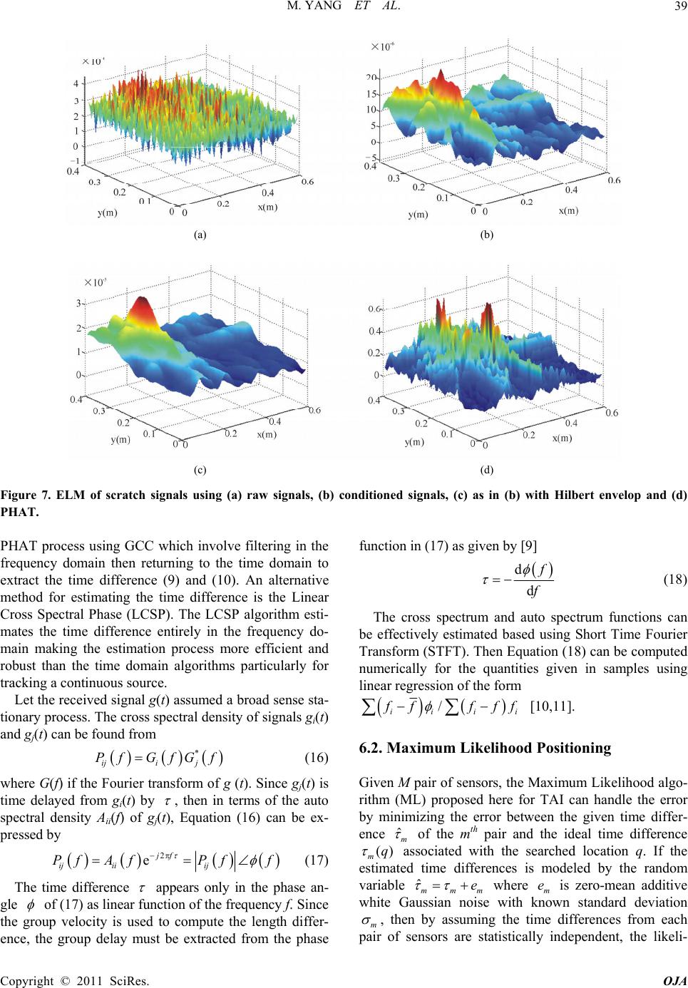

M. YANG ET AL. 39
(a) (b)
(c) (d)
Figure 7. ELM of scratch signals using (a) raw signals, (b) conditioned signals, (c) as in (b) with Hilbert envelop and (d)
PHAT.
PHAT process using GCC which involve filtering in the
frequency domain then returning to the time domain to
extract the time difference (9) and (10). An alternative
method for estimating the time difference is the Linear
Cross Spectral Phase (LCSP). The LCSP algorithm esti-
mates the time difference entirely in the frequency do-
main making the estimation process more efficient and
robust than the time domain algorithms particularly for
tracking a continuous source.
Let the received signal g(t) assumed a broad sense sta-
tionary process. The cross spectral density of signals gi(t)
and gj(t) can be found from

*
iji j
Pf GfGf (16)
where G(f) if the Fourier transform of g (t). Since gj(t) is
time delayed from gi(t) by

, then in terms of the auto
spectral density Aii(f) of gj(t), Equation (16) can be ex-
pressed by
 
2
ejf
ij iiij
P
fAfPf f



 (17)
The time difference

appears only in the phase an-
gle

of (17) as linear function of the frequency f. Since
the group velocity is used to compute the length differ-
ence, the group delay must be extracted from the phase
function in (17) as given by [9]

d
d
f
f

  (18)
The cross spectrum and auto spectrum functions can
be effectively estimated based using Short Time Fourier
Transform (STFT). Then Equation (18) can be computed
numerically for the quantities given in samples using
linear regression of the form




/
ii ii
f
ffff  

 [10,11].
6.2. Maximum Likelihood Positioning
Given M pair of sensors, the Maximum Likelihood algo-
rithm (ML) proposed here for TAI can handle the error
by minimizing the error between the given time differ-
ence ˆm

of the mth pair and the ideal time difference
()
mq

associated with the searched location q. If the
estimated time differences is modeled by the random
variable ˆmmm e



 where m e is zero-mean additive
white Gaussian noise with known standard deviation
m

, then by assuming the time differences from each
pair of sensors are statistically independent, the likeli-

M. YANG ET AL. 40
hood function can be expressed by the conditional prob-
ability density function given by [12]

2
2
ˆ [()]
2 12
1
1
ˆˆ
,, |e
2
mm
m
Mq
Mmm
pq


 




 (19)
taking the log of both sides of (19) yield
 



1
2
2
2
11
ˆˆ
ln, ,|
ˆ
1ln 2
22
M
MM
mm
m
mm
m
pq
q









(20)
The ML estimation of location q is the position that
maximizes the likelihood function (20) or equivalently
that minimizes the second term since the first term is not
a function of q which results in the following localization
criterion


2
2
1
ˆ()
argminMmm
MLq mm
q
Jq








 (21)
Here
M
L
J
is a weighted least error estimator. If no sta-
tistics considered or m

is the same for all sensor pairs,
then the denominator is constant and (21) is reduced to
the following formula
 
2
1
ˆˆ
argmin( )
M
MLqm m
m
Jq q 





 (22)
A significant difference between ML and ELM can be
observed that ML doesn’t suffer from side lobes but on
the cost of sharpness which means that the ML algorithm
provides more stability while ELM algorithm provides
higher accuracy. The similarity between the ML maps of
the impact and scratch signals is due to the dependence
of the ML algorithm on the time differences already es-
timated not on the signal themselves.
7. Conclusions
In this paper, the in-solid acoustic source localization is
developed based on measuring the time difference of
arrivals between spatially separated sensors. For efficient
operation of TAI with this approach, two methods are
proposed for the source localization. In the one-step
method the ELM performs the localization based on two
algorithms, one encounters time domain processing with
conventional post filtering and the other employs PHAT
filtering in the frequency domain. In the two-steps
method, TDOA values are found first using either GCC
or LCSP then based on these values the source is local-
ized using ML algorithm. The effect of dispersion is
treated by introducing Hilbert envelop smoothing. A
criterion is proposed to detect outlier estimations that can
happen from domestic noise as door shut.
8. Acknowledgements
This work was financed by the European FP6 IST Pro-
ject “Tangible Acoustic Interfaces for Computer Human
Interaction”. The support of the European Commission is
gratefully acknowledged.
9. References
[1] W. Rolshofen, D. T. Pham, M. Yang, Z. Wang, Z. Ji and
M. Al-Kutubi, “New Approaches in Computer-Human
Interaction with Tangible Acoustic Interfaces,” IPROMs
2005 Virtual Conference, May 2005.
[2] X. Wang, Z. Wang and B. O’Dea, “A TOA-Based Loca-
tion Algorithm Due to NLOS Propagation,” IEEE Trans-
actions on Vehicular Technology, Vol. 52, No.1, January
2003, pp. 112-116.
[3] S. Birchfield and D. Gillmor, “Fast Bayesian Acoustic
Localization,” Proceedings of the IEEE International
Conference on Speech and Signal Processing, Florida,
Vol. 2, May 2002, pp. 1793-1796.
[4] P. Aarabi and S. Zaky, “Robust Sound Localization Us-
ing Multi-Source Audiovisual Information Fusion,” El-
sevier, Information Fusion, Vol. 2, No. 3, 2001, pp. 209-
223. doi:10.1016/S1566-2535(01)00035-5
[5] C. Knapp and G. Carter, “The Generalized Correlation
Method for Estimation of Time Delay”, IEEE Transac-
tions on Acoustics, Speech, & Signal Processing Vol. 24,
No. 4, 1976, pp. 320-327.
doi:10.1109/TASSP.1976.1162830
[6] M. Omologo and P. Svaizer, “Acoustic Localization in
Noisy and Reverberant Environment Using CSP Analy-
sis,” Proceedings of the IEEE International Conference
on Acoustics, Speech, and Signal Processing Conference,
Atlanta, Vol. 2, 7-10 May 1996, pp. 921-924.
[7] J. Valin, F. Michaud, J. Rouat, D. LCtoumeau, “Robust
Sound Source Localization Using a Microphone Array on
a Mobile Robot,” Proceedings of the IEEE/RSJ Interna-
tional Conference on Intelligent Robots and Systems, Las
Vegas, 27-31 October 2003, Vol. 2, pp. 1228- 1233.
[8] J. Bendat and A. Piersol, “Random Data,” John Wiley &
Sons, 1986.
[9] A. Mertins, “Signal Analysis,” John Wiley & Sons, 1999.
[10] L. Danfeng and S. Levinson, “A Linear Phase Unwrap-
ping Method for Binaural Sound Source Localization on
a Robot,” Proceedings of the IEEE Conference on Ro-
botics and Automation, Washington, May 2002, pp. 19-
23.
[11] H. Poor, “An introduction to Signal Detection and Esti-
mation,” 2nd Edition, Springer, New York, Berlin, Hei-
delberg, Hong Kong, London, Milan, Paris, Tokyo, 1994.
[12] N. Gershenfeld, “The Nature of Mathematical Modeling”,
Cambridge University Press, Cambridge, 1999.