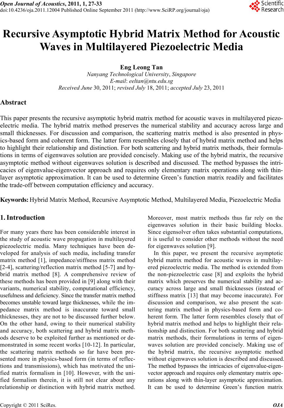Open Journal of Acoust i c s , 2011, 1, 27-33
doi:10.4236/oja.2011.12004 Published Online September 2011 (http://www.SciRP.org/journal/oja)
Recursive Asymptotic Hybrid Matrix Method for Acoustic
Waves in Multilayered Piezoelectric Media
Eng Leong Tan
Nanyang Technological University, Singapore
Received June 30, 2011; revised July 18, 2011; accepted July 23, 2011
Abstract
This paper presents the recursive asymptotic hybrid matrix method for acoustic waves in multilayered piezo-
electric media. The hybrid matrix method preserves the numerical stability and accuracy across large and
small thicknesses. For discussion and comparison, the scattering matrix method is also presented in phys-
ics-based form and coherent form. The latter form resembles closely that of hybrid matrix method and helps
to highlight their relationship and distinction. For both scattering and hybrid matrix methods, their formula-
tions in terms of eigenwaves solution are provided concisely. Making use of the hybrid matrix, the recursive
asymptotic method without eigenwaves solution is described and discussed. The method bypasses the intri-
cacies of eigenvalue-eigenvector approach and requires only elementary matrix operations along with thin-
layer asymptotic approximation. It can be used to determine Green’s function matrix readily and facilitates
the trade-off between computation efficiency and accuracy.
Keywords: Hybrid Matrix Method, Recursive Asymptotic Method, Multilayered Media, Piezoelectric Media
1. Introduction
For many years there has been considerable interest in
the study of acoustic wave propagation in multilayered
piezoelectric media. Many techniques have been de-
veloped for analysis of such media, including transfer
matrix method [1], impedance/stiffness matrix method
[2-4], scattering/reflection matrix method [5-7] and hy-
brid matrix method [8]. A comprehensive review of
these methods has been provided in [9] along with their
variants, numerical stability, computational efficiency,
usefulness and deficiency. Since the transfer matrix method
becomes unstable toward large thicknesses, while the im-
pedance matrix method is inaccurate toward small
thicknesses, they are not to be discussed further below.
On the other hand, owing to their numerical stability
and accuracy, both scattering and hybrid matrix meth-
ods deserve to be exploited further as mentioned or de-
monstrated in some recent works [10-12]. In particular,
the scattering matrix methods so far have been pre-
sented more in physics-based form (in terms of reflec-
tions and transmissions), which has motivated the uni-
fied matrix formalism in [10]. However, with the uni-
fied formalism therein, it is still not clear about any
relationship or distinction with hybrid matrix method.
Moreover, most matrix methods thus far rely on the
eigenwaves solution in their basic building blocks.
Since eigensolver often takes substantial computations,
it is useful to consider other methods without the need
for eigenwaves solution [9].
In this paper, we present the recursive asymptotic
hybrid matrix method for acoustic waves in multilay-
ered piezoelectric media. The method is extended from
the non-piezoelectric case [8] and exploits the hybrid
matrix which preserves the numerical stability and ac-
curacy across large and small thicknesses (instead of
stiffness matrix [13] that may become inaccurate). For
discussion and comparison, we also present the scat-
tering matrix method in physics-based form and co-
herent form. The latter form resembles closely that of
hybrid matrix method and helps to highlight their rela-
tionship and distinction. For both scattering and hybrid
matrix methods, their formulations in terms of eigen-
waves solution are provided concisely. Making use of
the hybrid matrix, the recursive asymptotic method
without eigenwaves solution is described and discussed.
The method bypasses the intricacies of eigenvalue-eigen-
vector approach and requires only elementary matrix ope-
rations along with thin-layer asymptotic approximation.
It can be used to determine Green’s function matrix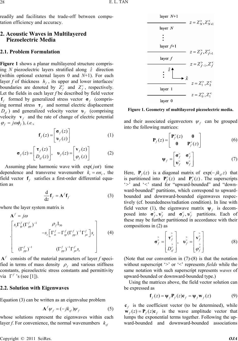

E. L. TAN 28
readily and facilitates the trade-off between compu-
tation efficiency and accuracy.
2. Acoustic Waves in Multilayered
Piezoelectric Media
2.1. Problem Formulation
Figure 1 shows a planar multilayered structure compris-
ing N piezoelectric layers stratified along ˆ z direction
(within optional external layers 0 and N+1). For each
layer f of thickness
f
h, its upper and lower interfaces/
boundaries are denoted by
f
Z
 and
f
Z
, respectively.
Let the fields in each layer f be described by field vector
f
f formed by generalized stress vector
f
σ (compris-
ing normal stress
f
τ and normal electric displacement
z
f
D) and generalized velocity vector
f
υ (comprising
velocity
f
v and the rate of change of electric potential
f
f
j



), i.e.,
()
() ()
f
ff
z
zz



σ
fυ (1)
() ()
(), ()
() ()
ff
ff
zf f
zz
zz
Dz z 
 

 
 
τv
συ (2)
Assuming plane harmonic wave with exp( )jt

time
dependence and transverse wavenumber tt ks

, the
field vector
f
f satisfies a first-order differential equa-
tion as
d
d
f
f
f
zfAf (3)
where the layer system matrix is
130
1
11
I
()
()
() ()
f
ff f
ttp pp
fff f
ttt tpppptt
fff
pppppt t
j
s
s
s
s


















A
(4)
f
A consists of the material parameters of layer f speci-
fied in terms of mass density
f

and various stiffness
constants, piezoelectric stress constants and permittivity
via
f
’s (see [1]).
2.2. Solution with Eigenwaves
Equation (3) can be written as an eigenvalue problem
()
f
f
zf f
jk

 A (5)
whose solutions represent the eigenwaves within each
layer f. For convenience, the normal wavenumbers
z
f
k
Figure 1. Geometry of multilayered piezoelectric media.
and their associated eigenvectors
f

can be grouped
into the following matrices:
()
() ()
f
ff
z
zz











P0
P0P (6)
f
f
f
f
f











σσ
ψυυ (7)
Here, ()
fzP is a diagonal matrix of exp( ) zf
jk z that
is partitioned into ()
fz

P and ()
fz

P. The superscripts
‘>’ and ‘<’ stand for “upward-bounded” and “down-
ward-bounded” partitions, which correspond to upward-
bounded and downward-bounded eigenwaves respec-
tively (cf. boundedness/radiation condition). In line with
field vector (1), the eigenwave matrix
f
ψ is decom-
posed into ,
f
f

συ and ,
f
f

συ partitions. Each of
these may be further partitioned in accordance with their
compositions in (2) as
,
f
f
ff
z
ff
D




















τv
συ (8)
(Note that our convention in (7)-(8) is that the notation
without superscript ‘>’ or ‘<’ represents field s while the
same notation with such superscript represents waves of
upward-bounded or downward-bounded type.)
Using the matrices above, the field vector solution can
be expressed as
() ()()
ffffff
zz z

fψPcψw (9)
f
c is the coefficient vector (to be determined), while
() ()
f
ff
zz

wPc is the wave amplitude vector that
lumps the exponential terms together. Following the up-
ward-bounded and downward-bounded associations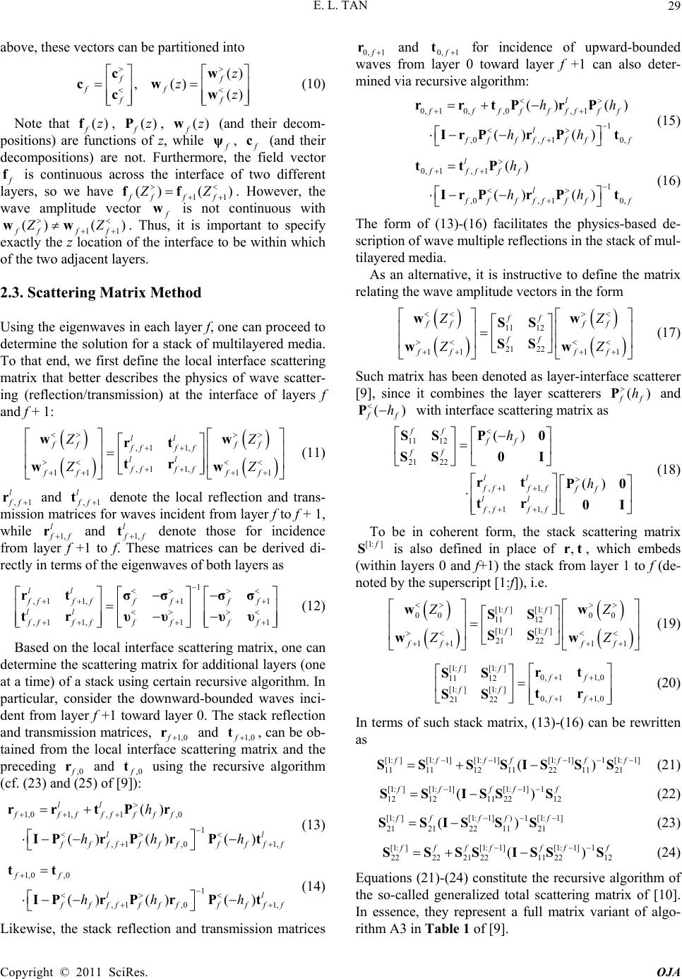

E. L. TAN 29
above, these vectors can be partitioned into
()
,() ()
ff
ff
ff
z
zz


 

 
 
 
cw
cw
cw
(10)
Note that ()
fzf, () fzP, () fzw (and their decom-
positions) are functions of z, while
f
ψ,
f
c (and their
decompositions) are not. Furthermore, the field vector
f
f is continuous across the interface of two different
layers, so we have 11 ()( )
fff f
ZZ


ff . However, the
wave amplitude vector
f
w is not continuous with
11
()( )
fff f
ZZ


ww . Thus, it is important to specify
exactly the z location of the interface to be within which
of the two adjacent layers.
2.3. Scattering Matrix Method
Using the eigenwaves in each layer f, one can proceed to
determine the solution for a stack of multilayered media.
To that end, we first define the local interface scattering
matrix that better describes the physics of wave scatter-
ing (reflection/transmission) at the interface of layers f
and f + 1:




,1 1,
,1 1,
11 11
ll
ff ff
fff f
ll
ffff
ff ff
ZZ
ZZ
 

 

 
 

 

 


 
ww
rt
tr
ww
(11)
,1
l
f
f
r and ,1
l
f
f
t denote the local reflection and trans-
mission matrices for waves incident from layer f to f + 1,
while 1,
l
f
f
r and 1,
l
f
f
t denote those for incidence
from layer f +1 to f. These matrices can be derived di-
rectly in terms of the eigenwaves of both layers as
1
,1 1,11
,1 1,11
ll
fff fffff
ll
ffffffff

 
 
 
 
 


 

 
 
rt σσ σσ
tr υυ υυ
(12)
Based on the local interface scattering matrix, one can
determine the scattering matrix for additional layers (one
at a time) of a stack using certain recursive algorithm. In
particular, consider the downward-bounded waves inci-
dent from layer f +1 toward layer 0. The stack reflection
and transmission matrices, 1, 0f r and 1, 0f t, can be ob-
tained from the local interface scattering matrix and the
preceding ,0
f
r and ,0
f
t using the recursive algorithm
(cf. (23) and (25) of [9]):
1,01,, 1,0
1
,1 ,01,
()
() ()()
ll
ffffffff
ll
f
ffff ffffff
h
hh h

 





 

rrtPr
IPr PrPt
(13)
1,0 ,0
1
,1 ,01,
() ()()
ff
ll
f
ffff ffffff
hh h






 

tt
IPr PrPt
(14)
Likewise, the stack reflection and transmission matrices
0, 1
f

r and 0, 1
f

t for incidence of upward-bounded
waves from layer 0 toward layer f +1 can also deter-
mined via recursive algorithm:
0, 10,,0, 1
1
,0, 10,
() ()
() ()
l
fffffffff
l
f
ffffff f
hh
hh





 

 

rrtP rP
IrPr Pt
(15)
0, 1, 1
1
,0, 10,
()
() ()
l
fffff
l
f
ffffff f
h
hh







 

ttP
IrPr Pt
(16)
The form of (13)-(16) facilitates the physics-based de-
scription of wave multiple reflections in the stack of mul-
tilayered media.
As an alternative, it is instructive to define the matrix
relating the wave amplitude vectors in the form





11 12
21 22
11 11
ff
ffff
ff
ff ff
ZZ
ZZ
 
 
 











ww
SS
SS
ww
(17)
Such matrix has been denoted as layer-interface scatterer
[9], since it combines the layer scatterers ()
f
f
h

P and
()
f
f
h
P with interface scattering matrix as
11 12
21 22
,1 1,
,1 1,
()
()
ff ff
ff
ll
fff fff
ll
fff f
h
h




 


 
 







SS P0
SS 0I
rt P0
tr 0I
(18)
To be in coherent form, the stack scattering matrix
[1: ]
f
S is also defined in place of ,rt, which embeds
(within layers 0 and f+1) the stack from layer 1 to f (de-
noted by the superscript [1:f]), i.e.





[1: ][1: ]
00 00
11 12
[1: ][1: ]
21 22
11 11
ff
ff
ff ff
ZZ
ZZ
 
 












ww
SS
SS
ww
(19)
[1: ][1: ]
0, 11,0
11 12
[1: ][1: ]
0, 11,0
21 22
ff ff
ff ff









rt
SS
tr
SS (20)
In terms of such stack matrix, (13)-(16) can be rewritten
as
[1:][1: 1][1: 1][1: 1]1[1: 1]
1111121122 11 21
()
ff fffff


 SS SSISSS (21)
[1: ][1:1][1:1]1
121211 2212
()
f
ffff
SSISS S (22)
[1:][1: 1])1[1: 1]
21 21 221121
()
fffff


SSISSS (23)
[1: ][1:1][1:1]1
222221 22112212
()
f
fffff f
 SSSSISS S (24)
Equations (21)-(24) constitute the recursive algorithm of
the so-called generalized total scattering matrix of [10].
In essence, they represent a full matrix variant of algo-
rithm A3 in Table 1 of [9].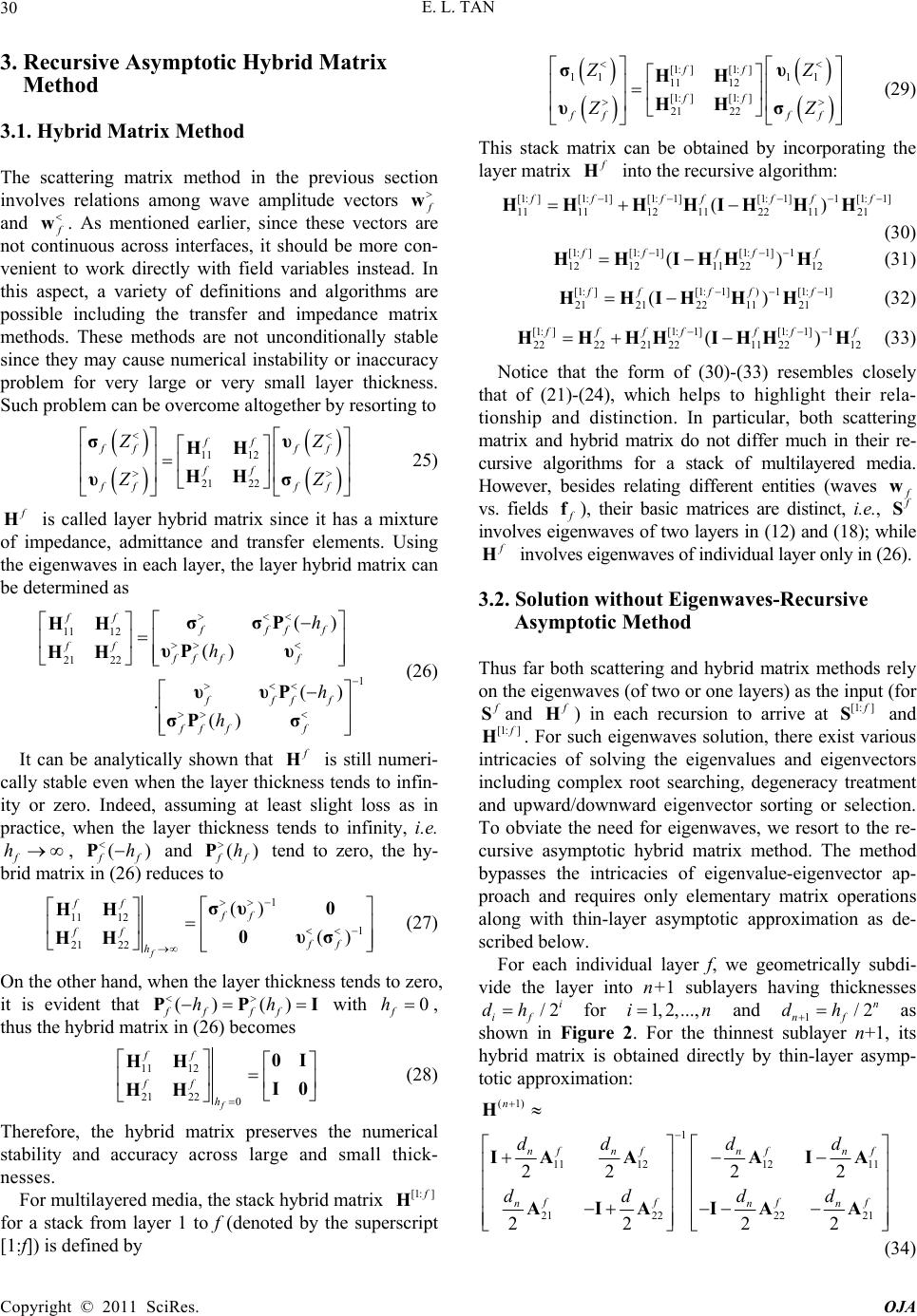

E. L. TAN 30
3. Recursive Asymptotic Hybrid Matrix
Method
3.1. Hybrid Matrix Method
The scattering matrix method in the previous section
involves relations among wave amplitude vectors
f

w
and
f

w. As mentioned earlier, since these vectors are
not continuous across interfaces, it should be more con-
venient to work directly with field variables instead. In
this aspect, a variety of definitions and algorithms are
possible including the transfer and impedance matrix
methods. These methods are not unconditionally stable
since they may cause numerical instability or inaccuracy
problem for very large or very small layer thickness.
Such problem can be overcome altogether by resorting to




11 12
21 22
ff
ff ff
ff
ff ff
ZZ
ZZ


 

 

 

 
συ
HH
HH
υσ
25)
f
H is called layer hybrid matrix since it has a mixture
of impedance, admittance and transfer elements. Using
the eigenwaves in each layer, the layer hybrid matrix can
be determined as
11 12
21 22
1
()
()
()
()
ff ffff
ff ff ff
ffff
ff ff
h
h
h
h

 


 

 










σσP
HH
υPυ
HH
υυP
σPσ
(26)
It can be analytically shown that
f
H is still numeri-
cally stable even when the layer thickness tends to infin-
ity or zero. Indeed, assuming at least slight loss as in
practice, when the layer thickness tends to infinity, i.e.
f
h, ()
f
f
h
P and ()
f
f
h

P tend to zero, the hy-
brid matrix in (26) reduces to
1
11 12
1
21 22
()
()
f
ff ff
ff ff
h










συ 0
HH
0υσ
HH (27)
On the other hand, when the layer thickness tends to zero,
it is evident that () ()
ff ff
hh

 PPI with 0
f
h

,
thus the hybrid matrix in (26) becomes
11 12
21 220
f
ff
ff
h







0I
HH
I0
HH (28)
Therefore, the hybrid matrix preserves the numerical
stability and accuracy across large and small thick-
nesses.
For multilayered media, the stack hybrid matrix [1: ]
f
H
for a stack from layer 1 to f (denoted by the superscript
[1:f]) is defined by





[1: ][1: ]
11 11
11 12
[1: ][1: ]
21 22
ff
ff
ff ff
ZZ
ZZ













συ
HH
HH
υσ
(29)
This stack matrix can be obtained by incorporating the
layer matrix
f
H into the recursive algorithm:
[1:][1: 1][1: 1][1: 1]1[1: 1]
1111121122 11 21
()
ff ff fff


 HH HHIHHH
(30)
[1: ][1:1][1:1]1
121211 2212
()
f
ffff
HHIHH H (31)
[1:][1: 1])1[1: 1]
212122 1121
()
fffff
HHIHHH (32)
[1:][1: 1][1: 1] 1
222221 2211 2212
()
f
ffffff
 HHHHIHH H (33)
Notice that the form of (30)-(33) resembles closely
that of (21)-(24), which helps to highlight their rela-
tionship and distinction. In particular, both scattering
matrix and hybrid matrix do not differ much in their re-
cursive algorithms for a stack of multilayered media.
However, besides relating different entities (waves
f
w
vs. fields
f
f), their basic matrices are distinct, i.e.,
f
S
involves eigenwaves of two layers in (12) and (18); while
f
H involves eigenwaves of individual layer only in (26).
3.2. Solution without Eigenwaves-Recursive
Asymptotic Method
Thus far both scattering and hybrid matrix methods rely
on the eigenwaves (of two or one layers) as the input (for
f
Sand
f
H) in each recursion to arrive at [1: ]
f
S and
[1: ]
f
H. For such eigenwaves solution, there exist various
intricacies of solving the eigenvalues and eigenvectors
including complex root searching, degeneracy treatment
and upward/downward eigenvector sorting or selection.
To obviate the need for eigenwaves, we resort to the re-
cursive asymptotic hybrid matrix method. The method
bypasses the intricacies of eigenvalue-eigenvector ap-
proach and requires only elementary matrix operations
along with thin-layer asymptotic approximation as de-
scribed below.
For each individual layer f, we geometrically subdi-
vide the layer into n+1 sublayers having thicknesses
/2
i
if
dh for 1, 2,...,in

and 1/2
n
nf
dh
 as
shown in Figure 2. For the thinnest sublayer n+1, its
hybrid matrix is obtained directly by thin-layer asymp-
totic approximation:
(1)
1
11 121211
212222 21
222 2
22 22
n
f
fff nnn n
ff ff
nnn
ddd d
ddd
d




 


 

 

 
 

 

 
H
IA AAIA
AIA IAA
(34)

E. L. TAN 31
x
z
Figure 2. Geometric subdivision of layer f into n + 1 sublay-
ers.
Starting with this matrix, we implement self-recursions
as
()(1)(1)(1)(1)(1) 1(1)
1111121122 1121
()
ii iiiii
 HH HHIHHH (35)
()(1)(1)(1) 1(1)
121211 2212
()
iiii i
HHIHH H (36)
()(1)(1)(1) 1(1)
212122 1121
()
iiii i
HHIHH H (37)
()(1)(1)(1)(1)(1) 1(1)
222221 22112212
()
ii iiiii
 HH HHIHHH (38)
This recursive algorithm proceeds until i = 1 and the
layer hybrid matrix is found as (1)fHH. Throughout
the procedure, there is no need to solve any eigenprob-
lem and the hybrid matrix can be computed stably and
accurately even for very thick or very thin layer.
4. Discussion and Numerical Results
The previous sections have discussed some algorithms
for scattering and hybrid matrix methods. For concise
comparison, Table 1 lists each of the algorithms and its
pertaining equations involved for each major step repre-
sented by an arrow. In each major step, there is at least
one (dense) matrix inversion to be dealt with, which of-
ten constitutes the most time-consuming operation. For
the scattering matrix method, we list the algorithms in
physics-based form as well as coherent form. The latter
form helps to bring out the close resemblance with the
algorithm of hybrid matrix method. Also listed in Table
1 is the input required for each algorithm. Since the scat-
tering matrix relates wave amplitude vectors across in-
terfaces, the input ought to be eigenwaves of two layers.
As for the hybrid matrix that relates field variables, the
input may need only the eigenwaves of individual layer.
Through the recursive asymptotic method, the input does
not invoke any eigenwaves at all.
To highlight the distinctions between the hybrid ma-
Table 1. Algorithms for scattering and hybrid matrix me-
thods.
Input Algorithm
Scattering matrix method:
 Physics-based form
(12)(13) (16)
1
,,,
ll
ff  ψψrtrt
 Coherent form
(12),(18)(21) (24)[1:]
1
,
f
f
ff  ψψ SS
With eigenwaves
(5) (7)
f
f

Aψ
Hybrid matrix method:
(26)(30) (33)[1: ]
f
f
f
ψHH
Without eigenwaves
(
f
A directly)
Recursive asymptotic hybrid matrix method:
(34) (38)(30) (33)[1:]
f
f
f
AHH
trix method with eigenwaves and the recursive asymp-
totic method without eigenwaves, we further list down
below the key steps in their respective procedure. In par-
ticular, the procedure with eigenwaves is
i) Solve the eigenvalue problem (5) for wavenumbers
and eigenvectors
ii) Perform upward/downward-bounded eigenvectors
sorting or selection in (6)-(7), noting the boundedness/
radiation condition and degeneracy treatment if needed
iii) Derive the layer hybrid matrix using (26).
Step i) is often time-consuming, while step ii) deserves
much careful attention and could be rather bothersome in
practice. On the other hand, the procedure without eigen-
waves via the recursive asymptotic method is
i') Initialize the thin-layer asymptotic approximation
(34) directly from
f
A
ii') Perform self-recursions (35)-(38) until i = 1
iii') The layer hybrid matrix is found as (1)f

HH.
All steps here are straightforward and involve elementary
matrix operations only.
To assess the accuracy of recursive asymptotic hybrid
matrix method, we investigate the relative error changes
with the number of geometric subdivisions n+1 or
equivalently, the recursion number n. We arbitrarily take
a ZnO layer of 1 μm thick at 1 GHz as an example. Fig-
ure 3 shows the average relative error versus recursion
number n. The relative error is measured by
-
ff f
ae e
HHH (39)
where
f
a
H and
f
e
Hrepresent the layer hybrid matrix
obtained from the recursive asymptotic method and ei-
genwaves solution, respectively. The error is calculated
by taking the average over a range of transverse wave-
numbers. Notice that the error decreases initially due to
smaller truncation error for smaller initial sublayer thick-
ness n d. After certain minimum point, the error in-
creases slightly and reaches a plateau without increasing
further.

E. L. TAN 32
Figure 3. Average relative error vs. recursion number n.
To illustrate the usefulness of recursive asymptotic
hybrid matrix method, let us consider a ZnO/ dia-
mond/Si structure at 2 GHz. The thicknesses of ZnO
and diamond layers are 1.2 and 10 μm respectively,
while Si substrate and vacuum are assumed semi-infi-
nite. For analysis of surface acoustic wave (SAW) on
such structure, one can derive the generalized Green’s
function matrix G defined by
() ()
()
NN NN
NN s
ZZ
Z 






vτ
G (40)
where
s

is the charge density on the surface. G
can be formulated using the scattering matrix with ei-
genwaves in a robust manner, see [5]. Alternatively, one
can also determine G using the stack hybrid matrix
[1: ]
N
H (for a stack from layer 1 to N) as

1
s0
s
diag(0,0,0,| |)
diag(1,1,1, 1)
t
js 

 
 
GIY
Y
(41)
where 0

is the permittivity for vacuum (layer N+1),
[1: ][1: ][1: ]1[1: ]
s2221 sub 1112
()
f
fff
 YHHZHH (42)
and sub Z is the characteristic surface impedance for Si
substrate (layer 0)
1
sub00
()

Zσυ (43)
The stack hybrid matrix [1: ]
N
H can be obtained
with or without eigenwaves solution as mentioned ear-
lier. Figure 4 shows the Green’s function element
44
||G computed with and without eigenwaves. In the
latter case, we apply the recursive asymptotic hybrid
matrix method with n=6. Although this recursion num-
ber is rather small, the results agree quite well and the
plots are barely distinguishable. Referring to Figure 3,
one can select higher recursion number for better accu-
Figure 4. Green function element computed with and with-
out eigenwaves (via recursive asymptotic hybrid matrix me-
thod with n = 6).
racy, although this may not be needed in many cases
(e.g. when material data is not that accurate). In gen-
eral, the computation efficiency is improved for lower
accuracy required and also for thinner layer with fewer
geometric subdivisions. Therefore the method provides
a very convenient way that facilitates the trade-off be-
tween computation efficiency and accuracy. Note that
the efficiency improvement here is meant for every
layer and one will gain substantial savings in the total
computation time when there are many layers in the
stack for modeling inhomogeneous media. Moreover,
the method is very useful for being simple enough
since it does not require any eigenwaves for all layers
(even semi-infinite substrate). Thus, it may be applica-
ble even when the eigensolver package is not readily
accessible, such as on light-weight multi-thread proc-
essors (e.g. GPUs).
5. Conclusions
This paper has presented the recursive asymptotic hy-
brid matrix method for acoustic waves in multilayered
piezoelectric media. The hybrid matrix method pre-
serves the numerical stability and accuracy across large
and small thicknesses. For discussion and comparison,
the scattering matrix method has also been presented in
physics-based form and coherent form. The latter form
resembles closely that of hybrid matrix method and
helps to highlight their relationship and distinction. For
both scattering and hybrid matrix methods, their for-
mulations in terms of eigenwaves solution have been
provided concisely. Making use of the hybrid matrix,
the recursive asymptotic method without eigenwaves

E. L. TAN 33
solution has been described and discussed. The method
bypasses the intricacies of eigenvalue-eigenvector ap-
proach and requires only elementary matrix operations
along with thin-layer asymptotic approximation. It can
be used to determine Green’s function matrix readily
and facilitates the trade-off between computation effi-
ciency and accuracy.
6. References
[1] E. L. Adler, “Matrix Methods Applied to Acoustic Waves
in Multilayers,” IEEE Transactions on Ultrasonics, Fe-
rroelectrics and Frequency Control, Vol. 37, No. 6, 1990,
pp. 485-490. doi:10.1109/58.63103
[2] B. Collet, “Recursive Surface Impedance Matrix Methods
for Ultrasonic Wave Propagation in Piezoelectric Multi-
layers,” Ultrasonics, Vol. 42, No. 1-9, 2004, pp. 189-197.
[3] L. Wang and S. I. Rokhlin, “A Compliance/Stiffness
Matrix Formulation of General Green’s Function and Ef-
fective Permittivity for Piezoelectric Multilayers,” IEEE
Transactions on Ultrasonics, Ferroelectrics and Fre-
quency Control, Vol. 51, No. 4, 2004, pp. 453-463.
[4] E. L. Tan, “Stiffness Matrix Method with Improved Effi-
ciency for Elastic Wave Propagation in Layered Anisot-
ropic Media,” Journal of the Acoustical Society of Amer-
ica, Vol. 118, No. 6, 2005, pp. 3400-3403.
doi:10.1121/1.2118287
[5] E. L. Tan, “A Robust Formulation of SAW Green’s
Functions for Arbitrarily Thick Multilayers at High Fre-
quencies,” IEEE Transactions on Ultrasonics, Ferroelec-
trics and Frequency Control, Vol. 49, No. 7, 2002, pp.
929- 936. doi:10.1109/TUFFC.2002.1020163
[6] E. L. Tan, “A Concise and Efficient Scattering Matrix
Formalism for Stable Analysis of Elastic Wave Propaga-
tion in Multilayered Anisotropic Solids,” Ultrasonics,
Vol. 41, No. 3, 2003, pp. 229-236.
doi:10.1016/S0041-624X(02)00447-X
[7] T. Pastureaud, V. Laude, and S. Ballandras, “Stable Scat-
teringmatrix Method for Surface Acoustic Waves in Pie-
zoelectric Multilayers,” Applied Physics Letters, Vol. 80,
No. 14, 2002, pp. 2544-2546. doi:10.1063/1.1467620
[8] E. L. Tan, “Hybrid Compliance-Stiffness Matrix Method
for Stable Analysis of Elastic Wave Propagation in Mul-
tilayered Anisotropic Media,” Journal of the Acoustical
Society of America, Vol. 119, No. 1, 2006, pp. 45-53.
doi:10.1121/1.2139617
[9] E. L. Tan, “Matrix Algorithms for Modeling Acoustic
Waves in Piezoelectric Multilayers,” IEEE Transactions
on Ultrasonics, Ferroelectrics and Frequency Control,
Vol 54, No. 10, 2007, pp. 2016-2023.
doi:10.1109/TUFFC.2007.496
[10] V. Y. Zhang and V. Laude, “Unified and Stable Scatter-
ing Matrix Formalism for Acoustic Waves in Piezoelec-
tric Stacks,” Journal of Applied Physics, Vol. 104, 2008,
064916.
[11] M. Lam, E. Le Clézio, H. Amorín, M. Algueró, Janez
Holc, Marija Kosec, A. C. Hladky-Hennion and G. Feuil-
lard, “Acoustic Wave Transmission through Piezoelectric
Structured Materials,” Ultrasonics, Vol. 49, No. 4-5,
2009, pp. 424-431.
[12] E. L. Tan, “Generalized Eigenproblem of Hybrid Matrix
for Floquet Wave Propagation in One-Dimensional Pho-
nonic Crystals with Solids and Fluids,” Ultrasonics, Vol.
50, No. 1, 2010, pp. 91-98.
[13] L. Wang and S. I. Rokhlin, “Modeling of Wave Propaga-
tion in Layered Piezoelectric Media by a Recursive As-
ymptotic Matrix Method,” IEEE Transactions on Ultra-
sonics, Ferroelectrics and Frequency Control, Vol. 51,
No. 9, 2004, pp. 1060-1071.
doi:10.1109/TUFFC.2004.1334839