Modern Economy, 2011, 2, 654-666
doi:10.4236/me.2011.24073 Published Online September 2011 (http://www.SciRP.org/journal/me)
Cotton Hedging: A Comparison across Developing and
Developed Countries
Qizhi Wang, Benaissa Chidmi
Ag. & Applied Economics, Texas Tech University, Lubbock, USA
Received April 26, 2011; revised June 15, 2011; accepted July 2, 2011
Abstract
This paper uses the results of ordinary least squares, bivariate vector autoregressive, and error correction
models to estimate the hedge ratios for cotton production across different countries and to determine whether
New York Cotton Exchange futures prices can serve as a hedging tool for cotton producers. Models com-
parison shows that the error correction model fits the data better. The results of the error correction model
show that the spot prices and the NYCE futures prices are co-integrated in United States, Australia, and
China, but not in Africa Franc Zone countries. In addition, for countries with higher market power, such as
US and China, and countries without market distortions, such as Australia, the New York Cotton Exchange
futures prices can serve as a hedging tool for cotton producers. In contrast, for less developed countries, such
as Africa Franc Zone countries, and Pakistan, the NYCE futures prices cannot serve as hedging tool against
the risks faced by cotton farmers.
Keywords: Cotton, Hedge Ratio, Error Correction Model
1. Introduction
Cotton is one of the major natural fibers. It accounts for
around 40 percent of the world’s annual textile fiber pro-
duction and serves as an engine of economic growth by
providing income to millions of farmers in both deve-
loped and developing countries worldwide. Between 1
and 2 million households produce cotton in West Africa,
and up to 16 million people are involved in cotton pro-
duction in some way (International Cotton Advisory
Committee, 2007). The contribution of cotton to national
gross domestic product (GDP) varies among countries.
For instance, cotton provides 3 to 5 percent of the GDP
in Benin, Burkina Faso, Mali, and Chad. In addition,
cotton’s exports generate significant resources for na-
tional economies. For example, in Burkina Faso, Benin,
Chad, Mali, and Togo, cotton export share in total ex-
ports represents 51.4 percent, 37.6 percent, 36.2 percent,
25 percent and 11.2 percent, respectively (Hussein,
Hitimana, and Perret, 2005) [1]. Cotton also plays an
important role in the United States. The United States
produces about 20 percent of the world’s cotton supply
and consumes about 10 percent of world cotton. Cotton
provides about 0.1 percent of U.S. GDP (Irwin, 2001) [2].
The importance of the cotton trade is also evident in that
much of the world’s cotton crosses international borders
more than once before reaching its final consumers
(MacDonald, 2000) [3].
In recent years, several policy and technology changes
in the textile industry have affected the cotton market
and world cotton trade. In 2005, world textile trade be-
gan to operate under the Agreement on Textiles and
Clothing (ATC) instead of the Multi Fiber Agreement
(MFA). Based on that new rule, all quotas in the cotton
textile industry were eliminated. In 2001, China was ad-
mitted into the World Trade Organization (WTO) and
became a major player in the textile industry. China has
continued to increase its share of world mill consumption,
which jumped from 27 percent in 2001 to 42 percent in
2008 (Foreign Agricultural Service (FAS), 2008) [4].
Another important change has been the dramatic in-
crease in grain prices that has accompanied the expan-
sion of biofuel production in the United States, Europe,
and South America. Because cotton must compete for
space with corn, soybeans, and other crops, it is reason-
able to think that planted areas of cotton in some major
cotton producing countries will decrease. This is indeed
the case in the US: the harvested areas of cotton de-
creased 7.8 percent in 2006/07 from 2005/06 levels, 17.6
percent in 2007/08 down from 2006/07, and 22.8 percent

Q. Z. WANG ET AL.655
in 2008/09, down from 2007/08 (FAS, 2008) [4]. The
total harvested areas of cotton decreased around 2.3 mil-
lion hectares, which is more than the total cotton har-
vesting area in the Africa Franc Zone countries. The in-
crease in India’s cotton production due to the adoption of
Bt cotton, which made India the second largest cotton
exporter in the world, with 24 percent of world cotton
trade (FAS, 2008) [4] is another key factor in cotton in-
dustry.
Finally, exchange rate volatility and monetary policy
in many countries influence cotton production and price
levels. For example, the devaluation of the CFA franc in
January 1994 by 100 percent against the French franc
boosted cotton production in CFA countries, augmented
by a strong U.S. dollar that climbed to a peak against the
Euro in February 2002. However, this trend has since
reversed, affecting the profitability of cotton production
in the African Franc Zone (Estur, 2004) [5]. Based on an
orderly correction in the US current account deficit in
2006, the World Bank expected an annual 5 percent ef-
fective decline in the US currency through 2008 (Busi-
ness News, 2006) [6].The long term depreciation of the
US dollar reflects the long term decline in commo- dity
prices, and also the world’s historically higher rates of
inflation. On the other hand, appreciation of Chinese
currency would also increase the cost of textile exports
and as a result, would decrease Chinese cotton imports.
These new trends in the world cotton market indicate that
the cotton price will remain volatile. Some of these
trends may cause an increase in the world price of cotton,
while others trends may reduce it.
World cotton prices have fluctuated widely in the last
sixty years. Figure 1 presents the world cotton Cotlook
A-index prices and the New York Cotton Exchange
(NYCE) near December contract price over the last 30
years. From Figure 1, one can see that both the Cotlook
A-index price and the NYCE near December contract
price follow the same pattern, with a low price of ap-
proximately 40 cents per pound in 2001/02 and a high of
around 94 cents per pound in 1994/95. During the most
recent 5 years, the price of cotton has been as low as
50.54 cents per pound in 2004/05 and as high as 73 cents
per pound in 2007/08.
Due to price volatility, some countries, such as those
in the Africa Franc Zone, are losing export earnings of
about $1 billion a year in direct and indirect costs as a
result of subsidies paid by the United States and Euro-
pean Union (World Trade Organization, 2003) [7]. At
the same time, exchange rate movements pose an addi-
tional risk to be managed, because of additional pressure
Figure 1. World Cotton A-Index and NYCE near December Contract.

Q. Z. WANG ET AL. 656
on cotton producers and exporters when exchange rates
are volatile. All these factors increase the exposure of the
African countries in particular, and less developed coun-
tries in general, to the risk involved in producing cotton.
Presently, cotton producers in developing countries
such as the African Franc Zone countries make very li-
mited use of risk management instruments to hedge their
exposure. Commodity cash prices are more variable than
futures prices. Futures and options may provide the most
efficient way to deal with short-term price uncertainty
(Varangis et al., 1994) [8]. In addition, futures and op-
tions contracts can allow more flexibility in selling deci-
sions. Therefore, hedging is useful in the cotton market.
There are, however several obstacles that must be over-
come in order to make use of hedging in The African
Franc Zone countries. First, the market in agricultural
products in both developed and developing countries is
not totally free and markets are not fully developed espe-
cially in developing countries. Second, there is a lack of
technical skills the use of risk management instruments
in developing countries. Although some governments
could make good use of hedging instruments to reduce
cotton price volatility, this practice only provides partial
coverage. Finally, the costs of hedging, i.e., the cost to
obtain data and information, may also impede the imple-
mentation of hedging policies.
A logical question that comes to the researcher and
policy maker’s mind is whether hedging instruments, as
used in developed countries, could be optimized to hedge
against the risks involved in producing cotton in less
developed and developing countries. Therefore, the ob-
jective of this paper is to determine the relationship be-
tween the NYCE cotton futures price and domestic farm
prices in African Franc Zone and other less developed
countries and compare it with the one prevailing in other
countries, such as the United States, China, and Australia.
This will shed light on how the changes in NYCE prices
are reflected in the changes in domestic prices, as well as
whether NYCE prices can be used to hedge cotton pro-
duction in these countries.
The rest of this paper is organized as follows. In the
next section, we present a conceptual framework. Section
three presents the methods and procedures used to esti-
mate the conceptual framework; while section four pre-
sents the data used. In section five, we discuss the find-
ings of the paper, and in section six we conclude.
2. Conceptual Framework
This section focuses on theoretical construction of the
hedging ratio. Cotton producers face substantial income
risk due to price fluctuations. Apart from government
price support schemes, such as counter cyclical payments,
the loan rate, and other programs as used in the United
States, a number of alternative market-based techniques
are practiced to deal with these income risks. For exam-
ple, farmers can spread their sources of income by culti-
vating various crops, or/and storing harvested outputs in
order to sell commodities during a high-price period in-
stead of a low-price period. It has been shown that stock-
holding is an important device for small holders to re-
duce price risks (Zant, 1998) [9].
A financial risk management instrument is a technique
that hedges price risks on futures exchanges. These types
of instruments have received increased attention in recent
policy discussions (World Bank, 1999) [10]. With re-
spect to the use of these instruments, questions such as
the costs of hedging price risks and the size of the wel-
fare gains to be obtained from using such tools are often
raised.
Consider a farmer who will harvest cotton at a known
date in the future. The price at which the cotton will be
sold at a given date is uncertain; hence, the profit from
cotton production is stochastic. We assume that the
farmers only consider the present and some future “ter-
minal” date. That is, the cotton producer is a myopic
agent (Johnson 1960 [11], Stein, 1961 [12], Holthausen,
1979 [13]) such that his decision horizon equals his
planning horizon. The farmer cannot revise his cash or
hedging position between the time of placing the hedge
and the time when it is liquidated. Based on these assum-
ptions, farmers’ production decisions are executed at two
distinct dates. At time 1, the output price is not known
with certainty. It is assumed that farmers can hedge the
risk associated with the output price uncertainty by
taking positions in the futures market. At time 2, the un-
certainty about the output price is resolved, and the far-
mers choose the level of hedging conditional on the open
futures and options position determined at time 1.
To compare the efficiency of different risk manage-
ment methods, especially whether farmers adopt the New
York near December contract crop year average cotton
price to hedge or not, the risk-minimizing strategies are
considered. It is assumed that farmers choose a best risk
management strategy based on a risk comparison among
different choices. That is, farmers will look at the addi-
tional risk of a given strategy relative to the optimal one.
Following Lence et al. (1993) [14], a benchmark in the
hedging literature is the static minimum variance hedge
ratio (SMV). The SMV is the proportion of the cash
position to be hedged in order to minimize the variance
of terminal wealth, for a given cash position. The SMV
is important, because it represents the optimal hedge
ratio for myopic agents who are extremely risk averse
(Ederington 1979 [15]; Kahl 1983 [16]).
Moreover, the SMV is the optimum hedge ratio when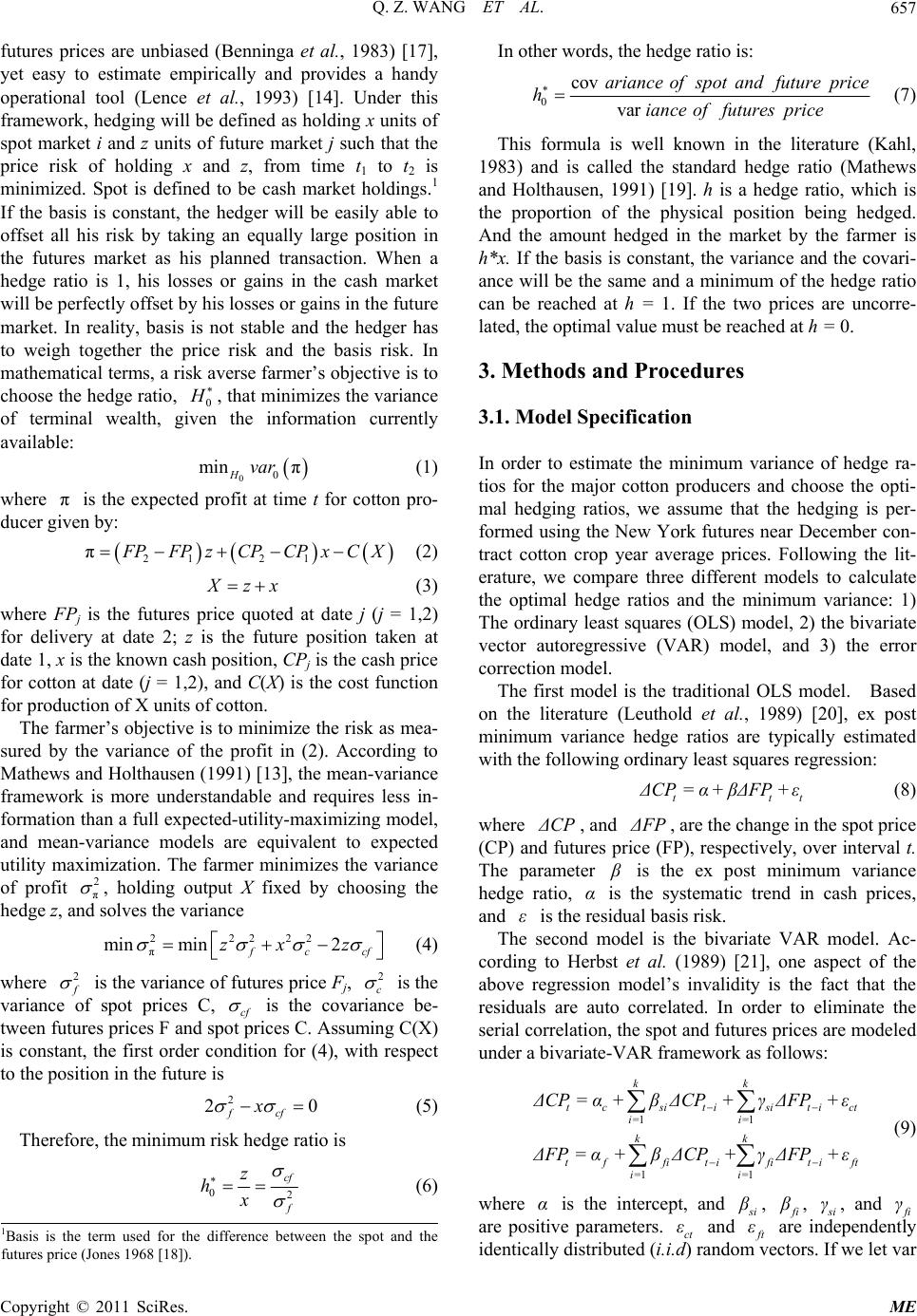

Q. Z. WANG ET AL.657
futures prices are unbiased (Benninga et al., 1983) [17],
yet easy to estimate empirically and provides a handy
operational tool (Lence et al., 1993) [14]. Under this
framework, hedging will be defined as holding x units of
spot market i and z units of future market j such that the
price risk of holding x and z, from time t1 to t2 is
minimized. Spot is defined to be cash market holdings.1
If the basis is constant, the hedger will be easily able to
offset all his risk by taking an equally large position in
the futures market as his planned transaction. When a
hedge ratio is 1, his losses or gains in the cash market
will be perfectly offset by his losses or gains in the future
market. In reality, basis is not stable and the hedger has
to weigh together the price risk and the basis risk. In
mathematical terms, a risk averse farmer’s objective is to
choose the hedge ratio, 0
H
, that minimizes the variance
of terminal wealth, given the information currently
available:

00
min π
Hvar (1)
where is the expected profit at time t for cotton pro-
ducer given by:
π





21 21
π
F
PFPzCPCPxCX   (2)
X
zx

 (3)
where FPj is the futures price quoted at date j (j = 1,2)
for delivery at date 2; z is the future position taken at
date 1, x is the known cash position, CPj is the cash price
for cotton at date (j = 1,2), and C(X) is the cost function
for production of X units of cotton.
The farmer’s objective is to minimize the risk as mea-
sured by the variance of the profit in (2). According to
Mathews and Holthausen (1991) [13], the mean-variance
framework is more understandable and requires less in-
formation than a full expected-utility-maximizing model,
and mean-variance models are equivalent to expected
utility maximization. The farmer minimizes the variance
of profit 2
π

, holding output X fixed by choosing the
hedge z, and solves the variance
22222
π
min min2
f
cc
zx z 



f



(4)
where 2
f

is the variance of futures price Fj, 2
c

is the
variance of spot prices C, cf

is the covariance be-
tween futures prices F and spot prices C. Assuming C(X)
is constant, the first order condition for (4), with respect
to the position in the future is
2
2
fcf
x  0

 (5)
Therefore, the minimum risk hedge ratio is
02
cf
f
z
hx


 (6)
In other words, the hedge ratio is:
0
cov
var
ariance ofspotandfutureprice
hiance offuturesprice
 (7)
This formula is well known in the literature (Kahl,
1983) and is called the standard hedge ratio (Mathews
and Holthausen, 1991) [19]. h is a hedge ratio, which is
the proportion of the physical position being hedged.
And the amount hedged in the market by the farmer is
h*x. If the basis is constant, the variance and the covari-
ance will be the same and a minimum of the hedge ratio
can be reached at h = 1. If the two prices are uncorre-
lated, the optimal value must be reached at h = 0.
3. Methods and Procedures
3.1. Model Specification
In order to estimate the minimum variance of hedge ra-
tios for the major cotton producers and choose the opti-
mal hedging ratios, we assume that the hedging is per-
formed using the New York futures near December con-
tract cotton crop year average prices. Following the lit-
erature, we compare three different models to calculate
the optimal hedge ratios and the minimum variance: 1)
The ordinary least squares (OLS) model, 2) the bivariate
vector autoregressive (VAR) model, and 3) the error
correction model.
The first model is the traditional OLS model. Based
on the literature (Leuthold et al., 1989) [20], ex post
minimum variance hedge ratios are typically estimated
with the following ordinary least squares regression:
t
ΔCP= α+βΔFP+ε
tt
(8)
where , and ΔCP
Δ
F
P, are the change in the spot price
(CP) and futures price (FP), respectively, over interval t.
The parameter
β
is the ex post minimum variance
hedge ratio, is the systematic trend in cash prices,
and is the residual basis risk.
α
ε
The second model is the bivariate VAR model. Ac-
cording to Herbst et al. (1989) [21], one aspect of the
above regression model’s invalidity is the fact that the
residuals are auto correlated. In order to eliminate the
serial correlation, the spot and futures prices are modeled
under a bivariate-VAR framework as follows:
11
11
kk
tcsit isit ict
i= i=
kk
tffitifiti ft
i= i=
ΔCP= α+βΔCP +γΔFP+ε
ΔFP= α+βΔCP+γΔFP+ ε




(9)
where is the intercept, and α
s
i
β
,
f
i, β
s
i, and γ
f
i
are positive parameters. ct and
γ
ε
f
t are independently
identically distributed (i.i.d) random vectors. If we let var
ε
1Basis is the term used for the difference between the spot and the
futures price (Jones 1968 [18]).

Q. Z. WANG ET AL. 658
(ct ε) =
s
s, var(σ
f
t) = ε
f
f , and cov(ct,σε
f
t) = ε
s
f,
many previous studies (Yang and Allen, 2005) [22] have
shown that the minimum variance hedge ratio is
σ
s
fff
s t
f
τ
+τ
hσσ
. (10)
The third model is the error-correction model. Based
on Ghosh (1993) [23], Lien and Luo (1994) [24] and
Lien (1996) [25], the second model described above ig-
nores co-integration between two price series. Accord-
ing to their suggestions, if two series are co-integrated, a
VAR model should be estimated along with the error-
correction term which accounts for the long-run equilib-
rium between spot and futures price movements. There-
fore the second model should be modified as follows:
1
1
t
Z+
Z+
11
11
kk
i
i=
kk
i
i=
+
+


ttsit ict
i=
ttfit ift
i=
=CP γΔFP +ε
=CP γΔFPε


c
f
α+
α+
si
fi
βΔ
βΔ
ΔCP
ΔFP


(11)
1t
Z
 is the error-correction term, which measures how
the dependent variable adjusts to the previous period’s
deviation from long-run equilibrium, according to the
following expression:
1
Z=
tt1
CP+δt1
F
P
 
(12)
where is the co-integrating vector. This two-variable
error-correction model expressed in equation (11) is a
bivariate VAR (k) model in first differences augmented
by the error-correction term 1
δ
s
t
τ
Z
 and 1
f
t
τ
Z

. The
coefficients
s
τ and
f
τ are interpreted as speed of ad-
justment parameters. The larger
s
τ is, the greater the
response of CP t to the previous period’s deviation from
long-run equilibrium.
3.2. Model Selection
In order to compare the performances of each type of
hedging strategy, the un-hedged portfolio is constructed,
consisting of shares with the same proportion as the
share price index held on the spot market. The hedged
portfolio is also constructed, consisting of a combination
of the share price index held on both the spot and the
futures markets. The number of futures contracts held is
determined by the computed hedge ratios from each
hedging strategy. The hedging performance is compared
in terms of the risk-return trade-off, and the percentage
variance reduction in the hedged portfolio relative to the
un-hedged portfolio.
According to Baillie and Myers (1991) [26], and Park
and Bera (1987) [27], the returns on the un-hedged port-
folio and the hedged portfolio are simply expressed as:
1ru CPtCPt (13)


11rhCPtCPthFPtPft

(14)
where ru and rh are return on un-hedged portfolio and
hedge portfolio, respectively. Ft and t are logged fu-
tures and spot prices at time period t, respectively, and
h* is the optimal hedge ratio. The return on the hedged
portfolio is the difference between the return on holding
the cash position and corresponding futures position.
Similarly, the variances of the un-hedged and the hedged
portfolios are expressed as:
C


2
c
Var U

 (15)


222
.
2
cf
Var Hhσhσ   
cf
(16)
where Var(U) and Var(H) represent variances of un-
hedged portfolio and hedged portfolio, respectively. c, σ
f
σ are standard deviation of the spot and futures price,
respectively; and c,f represents the covariance of the
spot and futures price.
σ
According to Ederington (1979) [15], the effectiveness
of hedging can be measured by the percentage of the
reduction in variance of the hedged portfolio relative to
the un-hedged portfolio. The variance reduction can be
calculated as:
 

Var UVarH
Var U
 (17)
The larger the variance reduction is, the better is the
hedging strategy. That is, the better hedging strategy
chosen has to provide more reduction of the variance
compared to the variance of the spot price in the cotton
market with the un-hedged strategy.
4. Data Sources and Estimation Issues
The data sets used in the studies come from different
sources. The primary data source is the cost of produc-
tion of raw cotton, published by International Cotton
Advisory Committee. Other sources include reports from
the USDA foreign Agricultural Service, Food and Agri-
culture Organization, the World Bank, and personal con-
tacts in the different countries.
Table 1 presents the descriptive statistics for the
twelve major cotton producers’ domestic farm prices
collected in the past thirty years, as well as the New
York Future market price. It shows that cotton price dis-
tributions are quite different among countries. The aver-
age cotton price in the United States, Australia and China
is closer to the New York Futures Market price; while
the Africa Franc Zone countries and Pakistan have a
lower average price than the other countries. Due to the
lack of record-keeping, there are only 28 years cotton
price data to collect from the Africa Franc zone countries
like Benin and Chad, and only 19 years of recorded cot-
ton prices for Brazil.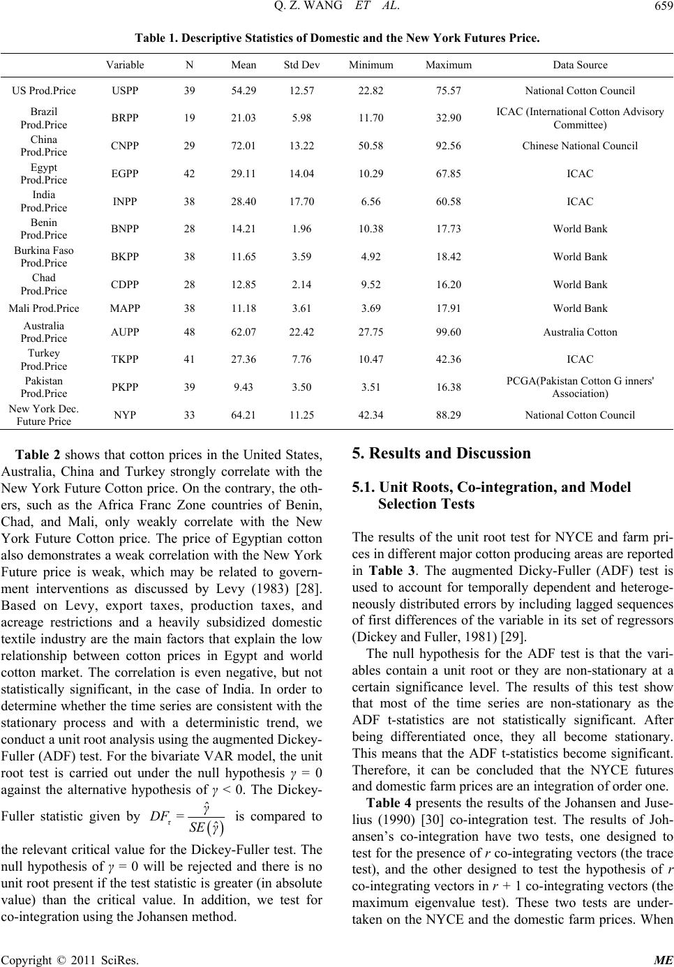

Q. Z. WANG ET AL. 659
Table 1. Descriptive Statistics of Domestic and the New York Futures Price.
Variable N Mean Std Dev Minimum Maximum Data Source
US Prod.Price USPP 39 54.29 12.57 22.82 75.57 National Cotton Council
Brazil
Prod.Price BRPP 19 21.03 5.98 11.70 32.90
ICAC (International Cotton Advisory
Committee)
China
Prod.Price CNPP 29 72.01 13.22 50.58 92.56 Chinese National Council
Egypt
Prod.Price EGPP 42 29.11 14.04 10.29 67.85 ICAC
India
Prod.Price INPP 38 28.40 17.70 6.56 60.58 ICAC
Benin
Prod.Price BNPP 28 14.21 1.96 10.38 17.73 World Bank
Burkina Faso
Prod.Price BKPP 38 11.65 3.59 4.92 18.42 World Bank
Chad
Prod.Price CDPP 28 12.85 2.14 9.52 16.20 World Bank
Mali Prod.Price MAPP 38 11.18 3.61 3.69 17.91 World Bank
Australia
Prod.Price AUPP 48 62.07 22.42 27.75 99.60 Australia Cotton
Turkey
Prod.Price TKPP 41 27.36 7.76 10.47 42.36 ICAC
Pakistan
Prod.Price PKPP 39 9.43 3.50 3.51 16.38 PCGA(Pakistan Cotton G inners' Association)
New York Dec.
Future Price NYP 33 64.21 11.25 42.34 88.29 National Cotton Council
5. Results and Discussion
Table 2 shows that cotton prices in the United States,
Australia, China and Turkey strongly correlate with the
New York Future Cotton price. On the contrary, the oth-
ers, such as the Africa Franc Zone countries of Benin,
Chad, and Mali, only weakly correlate with the New
York Future Cotton price. The price of Egyptian cotton
also demonstrates a weak correlation with the New York
Future price is weak, which may be related to govern-
ment interventions as discussed by Levy (1983) [28].
Based on Levy, export taxes, production taxes, and
acreage restrictions and a heavily subsidized domestic
textile industry are the main factors that explain the low
relationship between cotton prices in Egypt and world
cotton market. The correlation is even negative, but not
statistically significant, in the case of India. In order to
determine whether the time series are consistent with the
stationary process and with a deterministic trend, we
conduct a unit root analysis using the augmented Dickey-
Fuller (ADF) test. For the bivariate VAR model, the unit
root test is carried out under the null hypothesis γ = 0
against the alternative hypothesis of γ < 0. The Dickey-
5.1. Unit Roots, Co-integration, and Model
Selection Tests
The results of the unit root test for NYCE and farm pri-
ces in different major cotton producing areas are reported
in Table 3. The augmented Dicky-Fuller (ADF) test is
used to account for temporally dependent and heteroge-
neously distributed errors by including lagged sequences
of first differences of the variable in its set of regressors
(Dickey and Fuller, 1981) [29].
The null hypothesis for the ADF test is that the vari-
ables contain a unit root or they are non-stationary at a
certain significance level. The results of this test show
that most of the time series are non-stationary as the
ADF t-statistics are not statistically significant. After
being differentiated once, they all become stationary.
This means that the ADF t-statistics become significant.
Therefore, it can be concluded that the NYCE futures
and domestic farm prices are an integration of order one.
Table 4 presents the results of the Johansen and Juse-
lius (1990) [30] co-integration test. The results of Joh-
ansen’s co-integration have two tests, one designed to
test for the presence of r co-integrating vectors (the trace
test), and the other designed to test the hypothesis of r
co-integrating vectors in r + 1 co-integrating vectors (the
maximum eigenvalue test). These two tests are under-
taken on the NYCE and the domestic farm prices. When
Fuller statistic given by

ˆ
ˆ
τ
γ
DF= SE γ is compared to
the relevant critical value for the Dickey-Fuller test. The
null hypothesis of γ = 0 will be rejected and there is no
unit root present if the test statistic is greater (in absolute
value) than the critical value. In addition, we test for
co-integration using the Johansen method.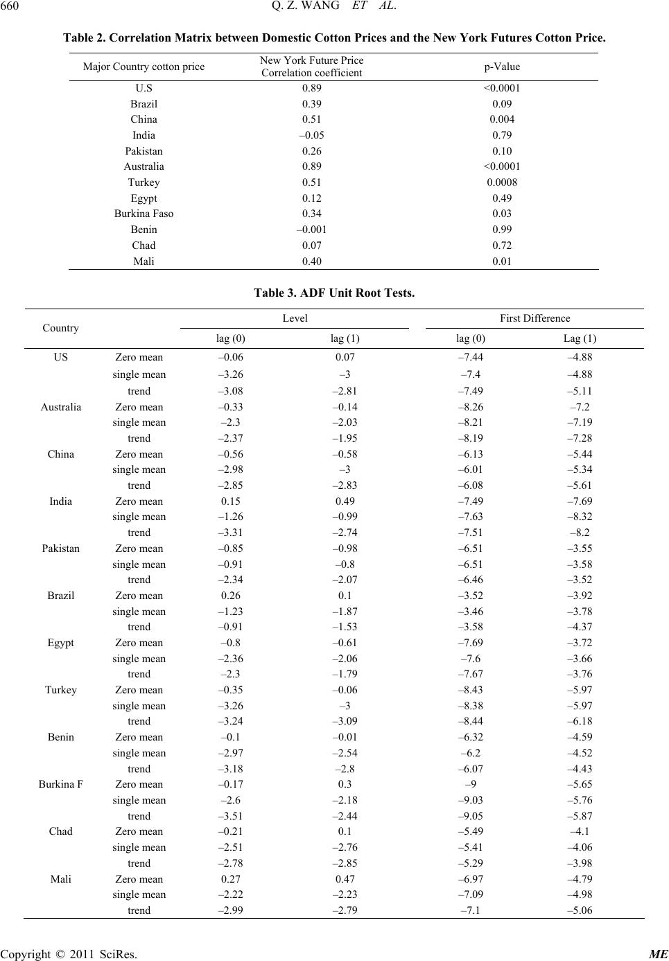

Q. Z. WANG ET AL. 660
Table 2. Correlation Matrix between Domestic Cotton Prices and the New York Futures Cotton Price.
Major Country cotton price New York Future Price
Correlation coefficient p-Value
U.S 0.89 <0.0001
Brazil 0.39 0.09
China 0.51 0.004
India –0.05 0.79
Pakistan 0.26 0.10
Australia 0.89 <0.0001
Turkey 0.51 0.0008
Egypt 0.12 0.49
Burkina Faso 0.34 0.03
Benin –0.001 0.99
Chad 0.07 0.72
Mali 0.40 0.01
Table 3. ADF Unit Root Tests.
Level First Difference
Country lag (0) lag (1) lag (0) Lag (1)
US Zero mean –0.06 0.07 –7.44 –4.88
single mean –3.26 –3 –7.4 –4.88
trend –3.08 –2.81 –7.49 –5.11
Australia Zero mean –0.33 –0.14 –8.26 –7.2
single mean –2.3 –2.03 –8.21 –7.19
trend –2.37 –1.95 –8.19 –7.28
China Zero mean –0.56 –0.58 –6.13 –5.44
single mean –2.98 –3 –6.01 –5.34
trend –2.85 –2.83 –6.08 –5.61
India Zero mean 0.15 0.49 –7.49 –7.69
single mean –1.26 –0.99 –7.63 –8.32
trend –3.31 –2.74 –7.51 –8.2
Pakistan Zero mean –0.85 –0.98 –6.51 –3.55
single mean –0.91 –0.8 –6.51 –3.58
trend –2.34 –2.07 –6.46 –3.52
Brazil Zero mean 0.26 0.1 –3.52 –3.92
single mean –1.23 –1.87 –3.46 –3.78
trend –0.91 –1.53 –3.58 –4.37
Egypt Zero mean –0.8 –0.61 –7.69 –3.72
single mean –2.36 –2.06 –7.6 –3.66
trend –2.3 –1.79 –7.67 –3.76
Turkey Zero mean –0.35 –0.06 –8.43 –5.97
single mean –3.26 –3 –8.38 –5.97
trend –3.24 –3.09 –8.44 –6.18
Benin Zero mean –0.1 –0.01 –6.32 –4.59
single mean –2.97 –2.54 –6.2 –4.52
trend –3.18 –2.8 –6.07 –4.43
Burkina F Zero mean –0.17 0.3 –9 –5.65
single mean –2.6 –2.18 –9.03 –5.76
trend –3.51 –2.44 –9.05 –5.87
Chad Zero mean –0.21 0.1 –5.49 –4.1
single mean –2.51 –2.76 –5.41 –4.06
trend –2.78 –2.85 –5.29 –3.98
Mali Zero mean 0.27 0.47 –6.97 –4.79
single mean –2.22 –2.23 –7.09 –4.98
trend –2.99 –2.79 –7.1 –5.06

Q. Z. WANG ET AL.661
Table 4. Johansen’s Co-integration Test.
Country H0 (rank = r) H1(rank > r) Eigenvalue value Test Trace Test Critical Value (5%)
US r = 0 r > 0 0.45 19.24* 12.21
r = 1 r > 1 0.01 0.29 4.14
China r = 0 r > 0 0.37 13.22* 12.21
r = 1 r > 1 0.01 0.25 4.14
Egypt r = 0 r > 0 0.17 5.98 12.21
r = 1 r > 1 0.01 0.19 4.14
India r = 0 r > 0 0.11 3.90 12.21
r = 1 r > 1 0.00 0.00 4.14
Australia r = 0 r > 0 0.45 19.52* 12.21
r = 1 r > 1 0.01 0.37 4.14
Turkey r = 0 r > 0 0.39 15.92* 12.21
r = 1 r > 1 0.01 0.28 4.14
Pakistan r = 0 r > 0 0.08 3.52 12.21
r = 1 r > 1 0.03 0.86 4.14
Brazil r = 0 r > 0 0.24 5.03 12.21
r = 1 r > 1 0.00 0.07 4.14
Benin r = 0 r > 0 0.42 14.96* 12.21
r = 1 r > 1 0.00 0.06 4.14
Burkina Faso r = 0 r > 0 0.33 12.69* 12.21
r = 1 r > 1 0.00 0.00 4.14
Chad r = 0 r > 0 0.35 11.79* 12.21
r = 1 r > 1 0.00 0.10 4.14
Mali r = 0 r > 0 0.25 9.22 12.21
r = 1 r > 1 0.00 0.03 4.14
the null hypothesis is that there is no co-integrating vec-
tor, both eigenvalue and trace statistics strongly reject the
null hypothesis. When the null hypothesis is that there is
a single co-integrating vector, both eigenvalue and trace
statistics fail to reject the null hypothesis.
Therefore, there is an indication of a co-integrating
relationship between the variables with rank of one. Af-
ter testing, it shows that the trace test values are greater
than critical values at the 5% level when the null hy-
pothesis is “r = 0”. The results imply that co-integration
exists in the US, China, Australia, Turkey and Benin.
When we test the rank value, it is insignificant or fails to
reject that the rank (H) is greater than 1 in the above
countries. In other words, we can say that there is co-
integration in the United States, China, Australia, Turkey
and Benin and we fail to reject that rank is equal to 1
based on the trace test. For Mali, Chad, Brazil and Paki-
stan, we fail to reject the co-integration relationship be-
tween those countries’ cotton prices and the NYCE fu-
tures price.
To test between the three models, this paper uses the
variance reduction procedure as explained in section 3.
Table 5 presents the results of the variance reduction.
Of the three constant hedge ratios derived from the OLS
model, the bivariate VAR model, and the error-corre-
ction model, the hedge ratio calculated from the OLS
regression model performs the worst in terms of reducing
portfolio variance, especially for major cotton players
such as the United States, China, Brazil, and Australia.
The error correction model gives the largest variance re-
duction for the United States, China, Brazil, and Austra-
lia. For the Africa Franc Zone countries, Egypt, Turkey,
Pakistan, India, and Brazil, there is a weak relationship
between domestic cotton prices and NYCE futures prices,
implying a non-statistically significant variance reduc-
tion as shown by the results.
The parameter estimates of the error correction model
are summarized in Table 6.2 The error correction models
were estimated by incorporating the error correction term
into the VAR model. For both equations of changes in
domestic farm prices and changes in futures price, the
coefficients of the error-correction term are statistically
2The results of the regression of the OLS and bivariate VAR models are
not presented here but can be obtained from the authors upon request.

Q. Z. WANG ET AL. 662
Table 5. Comparison of Variance Reduction from the Three Models.
Country V.R in OLS model V.R in VAR model V.R in Error correction Model
US 0.42 0.42 0.44
China 0.23 0.24 0.25
Brazil 0.11 0.12 0.15
Australia 0.22 0.23 0.29
Turkey 0.03 0.03 0.04
India –0.01 –0.03 –0.03
Pakistan 0.09 0.07 0.07
Egypt 0.01 0.01 0.01
Benin 0.00 0.00 –0.03
Burkina F 0.01 0.01 –0.03
Chad 0.00 0.00 –0.02
Mali 0.00 –0.01 0.00
Notes: Co-integration LR Test Based on Maximal Eigenvalue of the Stochastic Matrix and Trace of the Stochastic Matrix. r represents the number of linearly
independent co-integrating vectors.
Table 6. Estimated Hedging Ratios.
Hedge Ratio of country Number of Observation Traditional Model Bivariate VAR Model Error Correction Model
US 32 0.58 0.60 0.67
Australia 32 0.73 0.83 0.52
China 28 0.42 0.48 0.97
India 32 0.10 0.20 0.23
Pakistan 32 0.04 0.03 0.03
Brazil 18 0.10 0.10 0.15
Turkey 32 0.07 0.06 0.23
Egypt 32 0.20 0.17 0.17
Benin 27 –0.01 0.01 0.03
Burkina F 32 –0.04 –0.03 0.03
Chad 27 –0.02 0.00 –0.03
Mali 32 0.00 0.02 –0.01
significant, as indicated by the large values of the t-ratios.
The statistical significance of the long-run estimated pa-
rameter indicates that the error correction term is cor-
rectly signed in both equations and implies that spot
prices have a much greater speed of adjustment than the
futures price. The results of estimated long-run parame-
ters are significant in the US, China, Australia and Paki-
stan. The results indicate that there is co-integration be-
tween the spot prices in these countries and the NYCE
futures price.
We cannot, however, reach the same conclusion for
the Africa Franc Zone countries, Egypt, India, Brazil,
and Turkey. The results are not statistically significant in
these countries, we do not find any co-integration rela-
tionship and we cannot determine whether there exists
any long run relationship between the spot prices in these
countries and the NYCE futures price.
5.2. Hedge Ratio Results
Using the variance and covariance of the residuals, the
hedge ratios of the three models are calculated in Table
5. As expected, and in line with most of the previous
studies by Ghosh (1993) [23] and others, the hedge ratios
estimated by the error-correction model are greater than
those obtained from other models in most of the cases
except Australia. This is because co-integration exists
between futures prices and spot prices; ignoring this fact
would imply that the hedger should take a smaller than
optimal futures position.
In addition, the results indicate that countries with
higher market power such as the United States and China,
and countries without many market distortions, such as
Australia, have higher hedging ratios than the other
countries such as India, Turkey, Brazil and Egypt. On the

Q. Z. WANG ET AL. 663
Table 7. Estimate of the Error Correction model.
First Difference of Domestic Price First difference of New York future price
country Coefficient t-value Coefficient t-value
US Constant 0.28 0.19 0.71 0.37
∆CPt–1 –0.37 –1.21 0.41 1.08
∆FPt–1 0.32 1.29 –0.03 –0.11
LCPt–1 0.67 4.48 1.08 5.80
LFPt–1 –1.40 –4.48 –2.26 –5.80
Long-run Parameter beta
CP 1
FP –2.09 –2.07
Australia Constant –0.06 –0.03 0.66 0.35
∆CPt–1 –0.21 –1.29 0.61 4.06
∆FPt–1 0.49 2.24 –0.34 –1.72
LCPt–1 –0.12 –5.55 –0.10 –5.12
LFPt–1 –1.53 –5.55 –1.27 –5.12
Long-run Parameter beta
CP 1
FP 12.37 8.09
China Constant 0.31 0.09 0.51 0.20
∆CPt–1 –0.21 –0.72 –0.38 –1.79
∆FPt–1 –0.34 –1.13 0.14 0.61
LCPt–1 –0.32 –0.85 1.09 3.86
LFPt–1 0.46 0.85 –1.58 –3.86
Long-run Parameter beta
CP 1
FP –1.45 –3.15
India Constant 2.36 1.86 0.61 0.20
∆CPt–1 0.34 2.18 –0.67 –1.76
∆FPt–1 –0.21 –2.67 –0.50 –2.65
LCPt–1 –1.83 –6.63 0.33 0.49
LFPt–1 0.59 6.63 –0.11 –0.49
Long-run Parameter beta
CP 1
FP –0.32 –0.55
Pakistan Constant –0.02 –0.08 1.08 0.54
∆CPt–1 –0.63 –3.71 –3.96 –2.77
∆FPt–1 0.01 0.68 0.43 2.44
LCPt–1 0.12 1.76 4.00 6.95
LFPt–1 –0.06 –1.76 –1.97 –6.95
Long-run Parameter beta
CP 1
FP –0.49 –4.10

Q. Z. WANG ET AL. 664
Turkey Constant –0.06 –0.05 1.50 0.55
∆CPt–1 0.05 0.26 –0.89 –2.05
∆FPt–1 –0.27 –3.67 –0.21 –1.27
LCPt–1 –1.06 –3.76 2.15 3.46
LFPt–1 0.45 3.76 –0.92 –3.46
Long-run Parameter beta
CP 1
FP –0.42 –0.94
Brazil Constant 0.08 0.07 2.18 0.49
∆CPt–1 0.62 2.07 –0.67 –0.55
∆FPt–1 –0.12 –2.10 –0.47 –2.02
LCPt–1 –1.38 –4.13 0.22 0.16
LFPt–1 0.10 4.13 –0.02 –0.16
Long-run Parameter beta
CP 1
FP –0.07 –1.45
Egypt Constant –0.69 –0.33 0.30 0.14
∆CPt–1 –0.74 –5.17 –0.21 –1.45
∆FPt–1 0.17 1.03 0.31 1.81
LCPt–1 0.05 1.53 0.20 6.23
LFPt–1 –0.44 –1.53 –1.84 –6.23
Long-run Parameter beta
CP 1
FP –9.05 –0.23
Benin Constant 0.10 0.21 0.03 0.14
∆CPt–1 –0.54 –3.62 –2.31 –1.45
∆FPt–1 0.00 –0.10 0.19 1.81
LCPt–1 –0.13 –1.52 1.85 6.23
LFPt–1 0.10 1.52 –1.43 –6.23
Long-run Parameter beta
CP 1
FP –0.78 –1.28
Burkina Faso Constant 0.05 0.09 –0.19 0.01
∆CPt–1 –0.48 –3.69 –1.93 –3.38
∆FPt–1 –0.05 –1.13 0.10 1.07
LCPt–1 –0.36 –2.54 3.06 4.84
LFPt–1 0.16 2.54 –1.40 –4.84
Long-run Parameter beta
CP 1
FP –0.46 –1.87

Q. Z. WANG ET AL. 665
Chad Constant 0.02 0.04 0.23 0.10
∆CPt–1 –0.35 –2.07 0.55 0.64
∆FPt–1 0.05 1.34 0.28 1.55
LCPt–1 0.03 0.58 –1.54 –5.78
LFPt–1 0.03 0.58 –1.76 –5.78
Long-run Parameter beta
CP 1
FP 1.15 0.57
Mali Constant 0.04 0.11 1.05 0.48
∆CPt–1 –0.41 –2.55 0.38 0.44
∆FPt–1 0.08 2.80 0.09 0.55
LCPt–1 –0.14 –1.39 –2.70 –5.14
LFPt–1 –0.08 –1.39 –1.49 –5.14
Long-run Parameter beta
CP 1
FP 0.55 0.20
contrary, there is not much improvement or significant
change for the hedge ratios among the three regression
models for countries like Egypt and the Africa Franc
Zone countries. It can be concluded that for countries
that are without market power as well as subject to signi-
ficant domestic policy distortions, the NYCE futures
market price is not a good target for hedging. These re-
sults are consistent with Varangis et al. (1993) [8] who
find that the New York futures market does not provide
an appropriate mechanism for hedging the price risk in
Egyptian cotton.
6. Conclusions
This paper aims at estimating the hedge ratios for cotton
production across different countries and determining
whether New York Cotton Exchange futures prices can
serve as a hedging tool for cotton producers in these
countries. Three econometric models were used: ordinary
least squares, bivariate vector autoregressive, and error
correction models. The variance reduction test results
indicate that the error correction model outperforms the
ordinary least squares and the bivariate vector autore-
gressive models.
The results of the error correction model indicate that
spot prices have a much greater speed of adjustment than
the futures price. In addition, the results indicate that
there is co-integration between the spot prices and the
NYCE futures prices in the United States, Australia, and
China; while for Africa Franc Zone countries, the results
were not significant.
With respect to the hedge ratio, the findings of this
paper show that, overall, the hedge ratios implied by the
error correction model are larger than the ones implied
by the ordinary least squares and the bivariate VAR mo-
dels. The countries studied can, additionally, be grouped
into three categories based on the hedge ratios. In the
first, we find countries with higher market power, such
as the US and China, and countries without market dis-
tortions, such as Australia. For these countries, the New
York Cotton Exchange futures prices can serve as a hed-
ging tool for cotton producers as indicated by high hedge
ratio values. In the second category, we find developing
countries, such as Turkey, Brazil, India, and Egypt with
intermediate values of hedge ratios. Though the NYCE
futures prices cannot be used as a hedging tool for cotton
spot prices in these countries, we may conclude from the
results that in the future, the NYCE futures prices will
have a bigger impact. Finally, for less developed coun-
tries, such as Africa Franc Zone countries, and Pakistan,
the NYCE futures prices cannot serve as hedging tool
against the risks faced by cotton farmers.
7. References
[1] K. Hussein, L. Hitimana and C. Perret, “Cotton in West
Africa—The Economic and Social Stakes,” The Develop-
ment Dimension Series, OECD, Paris, 2005.
[2] D. Irwin, “Free Trade under Fire,” Princeton University
Press, New Jersey, 2002.
[3] R. MacDonald, “Concepts to Calculate Equilibrium Ex-
change Rates: An Overview,” Discussion Paper, Deut-
sche Bundesbank, Research Centre, Series 1, 2000.
[4] Foreign Agricultural Service, 2008.
http://www.fas.usda.gov/scriptsw/attacherep/default.asp

Q. Z. WANG ET AL. 666
[5] G. Estur, “Commodity Risk Management Approaches for
Cotton in West Africa,” 2004.
http://www.icac.org/cotton_info/speeches/estur/2004/com
_risk_man_04.pdf
[6] Business News, 2006.
http://business-school-blog.elliottback.com/34/world-bank-e
xpects-5-annual-depreciation-in-us-dollar-till-2000%20
[7] World Trade Organization, “Poverty Reduction: Sectoral
Initiative in Favor of Cotton,” Joint Proposal by Benin,
Burkina Faso, Chad, and Mali, Committee on Agriculture,
Special Session, TN/AG/GEN/4, May 16, 2003.
[8] P. Varangis, E. Thigpen and S. Satyanarayan, “The Use
of New York Cotton Futures Contracts to Hedge Cotton
Price Risk in Developing Countries,” Working Paper #
1328, Policy Research, 1994.
[9] W. Zant, “Stockholding, Price Stabilization and Futures
Trading: Some Empirical Investigations of the Indian
Natural Rubber Market. International Books van Arkel,”
Utrecht, Netherlands, 1998.
[10] World Bank, “Dealing with Commodity Price Volatility
in Developing Countries: A Proposal for a Market Based
Approach,” International Task Force on Commodity Risk
Management in Developing Countries, Washington, DC.
1999.
[11] L. L. Johnson, “The Theory of Hedging and Speculation
in Commodity Futures,” Review of Economic Studies,
Vol. 27, No. 3, 1960, pp. 139-151.
doi:org/10.2307/2296076
[12] J. L. Stein, “The Simultaneous Determination of Spot and
Future Prices,” American Economic Review, Vol. 59, No.
5, 1961, pp. 1012-1025.
[13] D. M. Holthausen, “Hedging and the Competitive Firm
under Price Uncertainty,” American Economic Review,
Vol. 69, No. 5, 1979, pp. 989-995.
[14] S. H. Lence, K. L. Kimle and M. L. Hayenga, “A Dy-
namic Minimum Variance Hedge,” American Journal of
Agricultural Economics, Vol. 75, No. 4, 1993, pp. 1063-
1071. doi:org/10.2307/1243994
[15] L. H. Ederington, “The Hedging Performance of the New
Futures Markets,” Journal of Finance, Vol. 34, No. 1,
1979, pp. 157-170. doi:org/10.2307/2327150
[16] K. H. Kahl, “Determination of the Recommended Hedg-
ing Ratio,” American Journal of Agricultural Economics,
Vol. 65, No. 3, 1983, pp. 603-605.
doi:org/10.2307/1240514
[17] S. Benninga, R. Eldor and I. Zilcha, “Optimal Hedging in
the Futures Market under Price Uncertainty,” Economic
Letters, Vol. 13, No. 2-3, 1983, pp. 141-145.
doi:org/10.1016/0165-1765(83)90076-9
[18] C. L. Jones, “Theory of Hedging on Beef Futures Mar-
ket,” American Journal of Agricultural Economics, Vol.
50, No. 5, 1968, pp. 1760-1766.
doi:org/10.2307/1237383
[19] K. H. Mathews and Holthausen, “A Simple Multi-Period
Minimum Risk Hedge Model,” American Journal of Ag-
ricultural Economics, Vol. 73, No. 4, 1991, pp. 1020-
1026. doi:org/10.2307/1242429
[20] R. M. Leuthold, J. C. Junkus and J. E. Cordier, “The
Theory and Practice of Futures Markets,” Lexington
Books, Lexington, MA, 1989.
[21] A. F. Herbst, D. D. Kare and J. F. Marshall, “A Time
Varying Convergence Adjusted Minimum Risk Futures
Hedge Ratio,” Advances in Futures and Options Re-
search, Vol. 6, 1993, pp. 137-155.
[22] W. Yang and D. Allen, “Multivariate GARCH Hedge
Ratios and Hedging Effectiveness in Australian Futures
Markets,” Accounting and Finance, Vol. 45, No. 2, 2005,
pp. 301-321. doi:org/10.1111/j.1467-629x.2004.00119.x
[23] A. Ghosh, “Co-Integration and Error Correction Models:
Intertemporal Causality between Index and Futures
Prices,” The Journal of Futures Markets, Vol. 13, No. 2,
1993, pp. 193-198. doi:org/10.1002/fut.3990130206
[24] D. D. Lien and X. Luo, “Estimating Multi-Period Hedge
Ratios in Co-Integrated Markets,” The Journal of Futures
Markets, Vol. 13, No. 8, 1993, pp. 909-920.
doi:org/10.1002/fut.3990130808
[25] D. D. Lien, “The Effect of the Co-Integrating Relation-
ship on Futures Hedging: A Note,” The Journal of Fu-
tures Markets, Vol. 16, No. 7, 1996, pp. 773-780.
doi:org/10.1002/(SICI)1096-9934(199610)16:7<773::AI
D-FUT3>3.0.CO;2-L
[26] R. T. Baillie and R. J. Myers, “Bivariate GARCH Esti-
mation of the Optimal Commodity Futures Hedge,”
Journal of Applied Econometrics, Vol. 6, No. 2, 1991,
pp. 109-124. doi:org/10.1002/jae.3950060202
[27] H. Y. Park and A. K. Bera, “Interest Rate Volatility, Ba-
sis, and Heteroscedasticity in Hedging Mortgages,” The
American Real Estate and Urban Economics Association
Journal, Vol. 15, No. 2, 1987, pp. 79-97.
[28] V. Levy, “The Welfare and Transfer Effects of Cotton
Price Policies in Egypt, 1965-1978,” American Journal of
Agricultural Economics, Vol. 65, No. 3, 1965, pp. 576-
580. doi:org/10.2307/1240509
[29] D.A. Dickey and W.A. Fuller, “Likelihood Ratio Statis-
tics for Autoregressive Time Series with a Unit Root,”
Econometrica, Vol. 49, No. 4, 1981, pp. 1057-1072.
[30] S. Johansen and K. Juselius, “Maximum Likelihood Es-
timation and Inference on Co-Integration with Applica-
tion to the Demand for Money,” Journal of Econometrics,
Vol. 53, No. 2, 1990, pp. 211-244.