Modern Economy, 2011, 2, 614-624
doi:10.4236/me.2011.24069 Published Online September 2011 (http://www.SciRP.org/journal/me)
Who Meets the Standrads: A Multidimensional Approach
Antonio Villar
Department of Economics, Pablo de Olavide Uni ve rsi t y & Ivie, Seville, Spain
Received June 9, 2011; revised July 15, 2011; accepted Ju ly 26, 2011
Abstract
We consider here the evaluation of the performance of a society with respect to a given set of targets. We
provide a characterization of an intuitive evaluation formula that consists of the mean of the shares of the
achievements in the targets. The criterion so obtained permits one not only to endogenously determine who
meets the standards and who does not, but also to quantify the degree of fulfilment. Two empirical illustra-
tions are provided: the compliance of the European Union Stability and Growth Pact, on the one hand, and
the evaluation of research excellence in the Spanish universities, on the other hand.
Keywords: Meeting the Standards, Bonus/Malus Criterion, Multidimensional Targets, Additive Monotonicity
1. Introduction
Consider an organization consisting of several units
whose performance is to be evaluated with respect to a
vector of targets or reference values previously set. De-
pending on the problem under consideration, those tar-
gets may represent absolute values, relative performance
thresholds, or a mixture of them. We can think that the
purpose of the evaluation is the allocation of some re-
sources among those who qualify and/or prestige or rec-
ognition. The evaluation procedure itself may be con-
ceived as a simple dichotomous criterion concerning the
achievement of the targets, it may attempt at providing
quantitative estimates of the overall degree of fulfilment,
or something in between (e.g. classification in different
categories).
We shall refer to the organization as a society and to
the incumbent units as agents. The key feature of the
problem is the existence of a society with many agents
whose performance is to be evaluated with respect to a
given set of multidimensional targets, to be called stan-
dards. Note that in some cases meeting the standards
may imply getting values below the thresholds.
Deciding who meets the standards in a multidimen-
sional scenario is not immediate. Two extreme positions
can be considered. On the one hand, there is the most
demanding interpretation by which meeting the standards
means achieving all target values simultaneously. On the
other hand, there is the other extreme interpretation ac-
cording to which achieving some target is a sufficient
criterion. Each of those polar views makes the decision
on who meets the standards rather trivial. The drawback
is that in both cases we may find very unfair outcomes,
as we can be treating equally highly different perform-
ances. The difficult problem is, of course, how to handle
the intermediate cases. That is, when agents in society
exceed some of the prescribed targets but fail to reach
some others (a relevant case in practice and a usual
source of conflicts). The bottom line is whether we admit
or not compensations among achievements, both across
dimensions and across agents, and what kind of com-
pensations should be considered (we shall refer to this
feature as the substitutability problem).
Let us consider two cases that illustrate well the key
features of this type of evaluation problem.
Example 1: The European Stability and Growth Pact
(SGP). The SGP is an agreement among the 16 members
of the European Union that take part in the Eurozone, to
facilitate and maintain the stability of the Economic and
Monetary Union. It involves setting reference values for
some key public finance variables and aims at enforcing
fiscal discipline after the monetary union (member states
adopting the euro have to meet the Maastricht convergence
criteria, and the SGP ensures that they continue to ob-
serve them). The basic reference values are two: (a) An
annual budget deficit no higher than 3% of GDP; (b) A
national debt lower than 60% of GDP. The question is:
Are the countries in the Eurozone complying with the
SGP?
Example 2: Research excellence in the Spanish
Universities. It is well known that Spanish universities
are not subject to regular evaluation processes, contrary

A. VILLAR615
to what happens to research groups or Faculty. As a
consequence, society tends to assume that all u niversities
are similar and the market does not discriminate gradu-
ates from different universities. Yet there are some data
that would allow evaluating the research performance of
the Spanish universities. The question is: Can we identify
the set of universities that excel in research, out of the
distribution of the results in the different research di-
mensions?
Those examples illustrate two specific cases of the
evaluation problem under consideration. In both exam-
ples the evaluation may require not only identifying
those who meet the standards, but also to estimate their
degree of success. In Example 1 the standards are fixed
externally whereas in Example 2 the standards are rela-
tive to the actual performance. Therefore, we can also
consider the question of whether some specific objec-
tives have been reached in Example 1, whereas this type
of question is meaningless in Example 2. Also observe
that meeting the standards in Example 1 means having
values of the index below the thresholds, whereas in
Example 2 it means values above the thresholds.
This type of problem can be regarded as a case of
multicriterion decision making (e.g. [1] and [2]). The
proposed solutions may be interpreted as a class of com-
promise solutions on specific domains that evaluate the
achievements in terms of some distance function (see, for
instance, [3] and [4]). Our approach, however, stems
from the principles that are applied for the analysis of
development, inequality and poverty. Roughly speaking
development measures allow to estimate the achieve-
ments, the targets play a similar role to the poverty thre-
sholds, and inequality enters the picture as measuring the
degree of substitutability among the achievements. See
[5-10].
The paper is organized as follows. Section 2 contains
the basic model. We present there the key assumptions
and the essential ideas of this contribution by means of a
simple and intuitive evaluation function: an arithmetic
mean of the shares of the achievements in the targets.
The axioms we use for that are rather standard: weighted
anonymity (any two agents with the same weight and the
same realizations are indistinguishable), weighted neu-
trality (all dimensions that enter with the same weight are
equally important), a normalization property, and addi-
tive monotonicity (an increase in the realizations entails
an increase in the evaluation function that depends posi-
tively on the size of that increment). Section 3 introduces
a more flexible evaluation model, allowing for different
degrees of substitutability between agents and dimen-
sions, by characterizing the uniparametric family of gen-
eralized means. Section 4 contains an empirical illustra-
tion of this approach by analyzing the two examples
presented above: the performance of the countries in the
Eurozone, regarding the EU Stability and Growth Pact,
and the selection of the set of excellent Spanish universi-
ties from a research viewpoint. A few final comments are
gathered in Section 5.
2. The Basic Model
2.1. Measuring the Achievements
Let


1, 2,,Nn
denote a society with agents
and let
n


1, 2,,
K
k
2
be a set of characteristics, with
. A realization is a matrix ij
Y with
rows, one for each agent, and columns, one for each
dimension. The entry ij
k



yn
k
y

 describes the value of
variable for agent . Therefore, is the space
of realization matrices and we assume implicitly that all
dimensions can be approximated quantitatively by real
numbers.
jink 
There is a parameter vector of reference values
k
z


 that describes the standards fixed for the dif-
ferent dimensions. We shall not discuss here how those
thresholds are set, even though the importance of that
choice is more than evident.
In order to deal with agents of different size or impor-
tance (e.g. families, firms, regions, countries), there is a
vector n



 that tells us the weights with which the
different agents enter into the evaluation. Similarly, in
order to allow for the presence of targets of different
merit, we introduce a vector that puts weights
on the different dimensions.
k



An evaluation problem, or simply a problem, is a point


,, ,PYz

 
We denote by
in the space nk knk
  
.


M
PN the set of agent
the standards in problem P.
s who meet
In order to evaluate the overall achievements of the
society with a realization matrix , relative to the refe-
rence vector , and weighting vectors
Y
z,


, we look
for a continuous function :

 that associates to
each problem P

 a real value that provides
a measure of its performance. This function is deter-
mined by a set of intuitive and reasonable properties that
we introduce next.

P


The first property we consider, weighted anonymity,
establishes that all weighted agents are treated alike. That
is, if we permute agents’ realization vectors together with
their associated weights, the evaluation does not change.
Weighted Anonymity: Let and let

,, ,Yz  




π,πY

denote a permutation of the indices of the
rows of matrix and the corresponding entries of
vector
Y

. Then,




,, ,π,,π,YzY z
 
.

A. VILLAR 616
The second property, weighted neutrality, says that all
weighted dimensions are equally important. That can be
expressed, in line with the definition above, as follows:
Weighted Neutrality: Let and let

,, ,Yz  
 
,Y

 denote a permutation applied to the indi-
ces of the columns of matrix and the corresponding
entries of vectors and
Y
z

. Then,
 
,, ,,,,YzY z


.
Next property, normalization, makes the value of the
index equal to zero when Y

0 (the null matrix) and
equal to i
iNjK j





,

when (where YZ

,,
Z
zzz
z
is the matrix whose columns repeat the
target vector for each agent).1 Formally:
Normalization:
 
,, ,0,,, ,i
iN jK
zZz j
 



0.
Our last property, additive monotonicity, establishes
conditions on the behaviour of the evaluation function
when the matrix of the agents’ achievements changes
from to , for some . The
property requires the change of the index to be a mono-
tone function
YYY Y
 nk
Y
g
of the change in the realization
matrix. This is a very natural property that is most useful
when the data on the agents’ performance is collected
from several sources, or across different time periods, or
when there are mistakes to be corrected. The new data
can be integrated by simply computing the value of that
function
Y
g
regarding those new data and adding up the
result to the original value of the index. Formally:
Additive Monotonicity: Let and let
. Then,

,, ,Yz  
nk
Y
  
,, ,,, ,,, ,YYzYz gYz

 
 
for some increasing function . :g
Note that this requirement is cardinal in nature and
involves a separability feature of the overall index. In-
deed, it implies that increasing the achievement of an
agent in a given dimension by one unit will have the
same impact on the index, no matter the level at which
this happens (perfect substitutability of weighted agents
and weighted dimensions).2
Remark It is easy to see that additive monotonicity
and normalization together imply additivity, that is,
  
,, ,,, ,,, ,YY zYzYz
The following result shows that all those requirements
yield an evaluation function that corresponds to the arith-
metic mean of the weighted shares of the achievements
in the targets. Formally:
Theorem 1: A continuos function :

 satis-
fies weighted anonymity, weighted neutrality, normaliza-
tion, and additive monotonicity, if and only if it takes the
form:

,, ,ij
ij
iNjK
j
y
Yz z  

 (1)
Moreover, those properties are independent.
Proof
1) The function in (1) satisfies all those properties. We
prove now the converse.
Let


,, ,PYz 

 and let be a
matrix with all elements other than equal to zero
and the

nk
ij a

,ij


,ij entry equal to . a
By applying repeatedly additive monotonicity we can
write:
 

,, ,
ij ij
iNjK
Pgyz




Let now


,,, a11 1a denote a uniform matrix whose
generic element is and take ,
zs1p


1,
d


1, for some positive scalars ,,
s
pd where 1 is
the unit vector in the corresponding space. Note that, in
this special case and in view of the weighted anonymity
and weighted neutrality properties, we have:
 
,, ,,, ,,
,,,
ij ht
g
aspdgaspd
ij Nht K

 
 

11 111 1
Therefore, we can write:






 
,,,,,
,, ,
,, ,
,,,,,
ij
ij
aspd
kngasp d
gaspd
aspd
nk











11111
11 1
11 1
11111


From that it follows:


  .


 
,, ,
1,,,,,
ijji j
iNjK
Yz
yz
nk




 11 111
(2)
Now observe that our assumptions imply that

is
linearly homogeneous, that is,


,, ,,, ,Yz Yz


  ,
for all 0

. Let now be given by:
4
:f  






: ,
ij jijijjij
fy,,,z,,, ,yz
 
111 11. As
1This simply extends the idea that the index is equal to one when Y = Z
and all agents and all targets are equally important, i.e. 1
in
 for
all , iN1
jk
 , for all . kK
2This property may have an ethical content when agents are made o
f
several individuals (e.g. the branches or the divisions of a firm) and the
evaluation involves some rewards. It ensures the neutrality of the rule
with respect to the order in which data are computed.

A. VILLAR617
this function inherits the linear homogeneity property
and satisfies normalization, by taking and
ij j
yz
ij
j
y
Z
 , we have:
,,
ij ij
jji ij
j
j
yy
fzz nk
zz






Therefore, plugging those values into Equation (2), for
all , we get: ,ij

,, ,ij
ij
iNjK
j
y
Yz z  






2) To separate the properties let us consider the fol-
lowing indices, for 1
in

 for all (anonymity), i
1
jk

 for all (neutrality):
j
2,a) 11 ,, ,ij
A
iNjK
j
y
Yz nk z 






11 . It satisfies
anonymity, neutrality, and additive monotonicity but not
normalization.
2,b) 11 ,, ,minij
BiN j
y
Yz nk z 


 





11 . It satisfies
anonymity, neutrality, and normalization but not additive
monotonicity.
2,c) 11 1
,, ,ij
Ci
iNjK
j
y
Yz nk kz 




 
 

11  , with
1
i
 
iN and 1
in

 for some i. It satisfies neu-
trality, normalization, and additive monotonicity but not
anonymity.
2,d) 11 1
,, ,ij
Dj
iNjK
j
y
Yz nk nz





 
 

11 

, with
1
j
jK


 and 1
jk

 for some . It satisfies
anonymity, normalization, and additive monotonicity but
not neutrality. Q.e.d.
j
This theorem tells us that assuming weighted anonym-
ity, weighted neutrality, normalization, and additive mo-
notonicity amounts to measuring social performance as
the (weighted) arithmetic mean of the agents’ relative
achievements.
It is interesting to observe that equation (2) provides
an implicit estimation of the performance of agent
with respect to dimension ,
i
j


,, ,
ij
eYz

 , that is
given by the evaluation of a fictitious society with a uni-
form realization matrix


,, ij
y
11, a uniform reference
vector
j
z1, and a uniform weighting system i

1,
j

1.
That is,
 


,, ,,,,,,
ij iijjij
eyzy z
This allows us to estimate the overall contribution of
an agent, by simply computing:
 

1
,, ,,,,,
ii
jK
ij
ij
jK j
CYzy z
k
y
nz
jji
 







11 11
(4)
that is, as i n

times the weighted sum of all her relative
achievements. Trivially, when 1
in

 we have the
weighted sum of the ijj yz values.
Similarly, we can have a measure of the overall suc-
cess of society in a given dimension, as:3

 


,, ,,,,,
j
ij jj
iN
ij
ji
iN j
SYzy z
y
kz
 







11 11
(5)
2.2. The Agents Who Meet the Standards and
the Targets that Have Been Reached
Let us consider now the question of who meets the stan-
dards and whether we can consider that a given target
has been collectively achieved. In our model those prob-
lems are solved endogenously by the very formula that
measures the overall performance. In order to facilitate
the exposition, we focus on the case in which meeting
the standards means achieving values above the estab-
lished thresholds. In that case, an agent with ,
for all , certainly meets the standards.
ij j
yz
j
Consider now an agent in the limit case in which
hj j
h
yz

, for all jK

. According to equation (3), the
overall performance of this agent is given by:




,,,,
hh h
jK
CYzznj

 


(where


,
h
Yz

z describes a matrix whose th row is
precisely ). Therefore, the set M(P) of agents who
meet the standards in problem is given by:
h
P

ij
jj
jK jK
j
y
MPiNz 





 






(6)
(note that we allow for the existence of agents in M(P)
whose achievements are below the target in some dimen-
sion, provided they are compensated with over compli-
ance in other dimensions).
Equation (6) permits one to directly identify the set of
those who meet the standards in the -dimensional
space in which we plot on all agents’ vectors of
k
k



11 111 (3)
3Note that computing the success in a given dimension makes sense
when the thresholds are externally given and may not be meaningful
when they correspond to functions of the actual values of the realiza-
tion matrix.

A. VILLAR 618
relative achievements,
 
1112 22
,,,,
iiikikk
y
zyzyzy   z,
for all . Indeed, the set iN

M
P
ij
yz
is given by all those
agents whose vectors of relative achievements are above
the hyperplane defined by

j
jK jK




k

.
When the reference values  are externally
given (i.e. they correspond absolute thresholds), we can
also consider whether a specific objective has been
reached by society. According to equation [5], objective
is achieved provided:
z
j

 
,, ,,1,, ,
j
jijj
iN
SYzS Yz z
 



,
where

,
j

j
Yz
1 describes a matrix whose th col-
umn is equal to
j
j
z in all entries. Therefore, the set of
objectives that have been collectively achieved are those
that satisfy the following condition:
,
ij
ii
iN iN
j
yjK
z



 (7)
3. A More Flexible Formlation
The additive structure of the evaluation function

in
Theorem 1 implies a particular trade-off between the
different achievements, as the evaluation only depends
on the sum of the agent's relative realizations but not on
their distribution. So each agent can substitute any rela-
tive realization for another one at a constant rate (equal
to ,
j
t

 for all ) no matter the level at
which this happens. Similarly, the relative achievements
of one agent in a given dimension can be substituted by
those of another one, once more at a constant rate (here
we find a marginal rate of substitution equal to
,jtK
ih


for all ). ,ihN
One might be willing to consider evaluation criteria
that incorporate variable degrees of substitutability (e.g.
decreasing marginal rates of substitution which implies
penalizing the inequality of realizations across agents
and/or dimensions, which may actually be a reason to
introduce such a criterion). The simplest way of allowing
for variable substitutability across agents and dimensions
is by looking for a uniparametric extension of the for-
mula in Theorem 1, so that controlling a single number
permits one to regulate the degree of substitutability. To
arrive at such a formula, let us start by performing the
following exercise. Let


,, ,PYz  
0
ij
y

 
ij
ij
iN jKj
y
Pz

 






The parameter

controls the impact of the individ-
ual deviations of the targets on the evaluation index. The
larger the value of

the larger the impact of values
above the reference level and viceversa. In particular, the
parameter

controls the degree of concavity (for
1


) or convexity (for 1

) of the function.
Note that we require for all entries of matrix
, in order to avoid inconsistencies. We therefore, set
0
ij
y
k
Ynk kn


 

 as our reference space from
now on.
What should be the relationship between the evalua-
tion of problems


P

and ? The following prop-
erty answers that question:
P

-Power: Let

,, ,PYz 

 and let








,  ,,PYz 

 y
denote a problem de-
rived from the previous as follows. Each ij in is
substituted by
Y


ij
y

and each
j
z z in is substituted
by


j
z

, for


. Then,
  
PP
1/







This property mimics the principle applied by the
variance to the measurement of differences to the mean.
If we take the power

of all relevant parameters of
the problem, then we re-scale the resulting formula by
taking the inverse power.
The following result is trivially obtained:4
Theorem 2: An index: 



 satisfies weighted
anonymity, weighted neutrality, “normalization”, addi-
tivity and

-power, if and only if it takes the form:

1/
,0
,
,0
ij
ij
ij
iN jKj
ij
iN jK j
y
z
Yz
y
z



 






















(8)
Moreover, those properties are independent.
Theorem 2 identifies the generalized mean of order

as the right formula to evaluate the performance of
the society, where

is the parameter that incorporates
our concern for equality across agents and dimensions
(or the degree of substitutability).
Remark Theorem 1 is not a particular case of Theo-
rem 2 becaus e the domain on which the evaluation func-
tion is defined is different.
, be a prob-
lem with strictly positive (i.e. for all )
and consider the transformation
Y,ij

Y

of Y given by


ij
yy

ij

 

z, for all , and the transformation ,ij

of vector given by j
The set of those who meet the standards is now given
z
 
j
zz

  for all ,
some scalar
j

. Call

P

to this transformed prob-
lem. Applying Theorem 1 to

P

we get:
4The first part of the normalization property has to be adjusted to the
new domain, by letting


0
lim, 0
YY

. We call “normalization”
(with inverted commas) to this modified property.

A. VILLAR619
by all agents whose vectors of weighted relative realiza-
tions, , are above (resp. below) the hy-
per-surface defined by:

,k
i
yz 



j
ij jj
jK jK
yz





.
Therefore, choosing

(the elasticity of substitution)
amounts to fix the bonus/malus frontier. In particular,

 (resp.

) corresponds to the extreme
case in which an agent meets the standards when she is
above the targets in all dimensions simultaneously (resp.
above some target); that is, the max (resp. the min) func-
tion. As for the intermediate cases, we find two of spe-
cial relevance: the arithmetic mean, associated to the
value 1

, discussed in the former section, and the
geometric mean, associated to the value 0

. A simi-
lar reasoning applies to the case of achieving some target,
with respect to the hyper-surface
ij
ii
iN iN
j
y
z









.
From a different viewpoint the parameter

may be
regarded as an equality coefficient in the following sense:
the smaller the value of

the more weight we attach
to a more egalitarian distribution of the agents’ achieve-
ments, both among themselves and with respect to the
different dimensions. The case 1

 shows no concern
for the distribution, as only the sum of the achievements
matters (inequality neutrality). Values of

smaller
than one correspond to inequality aversion. The geomet-
ric mean, in particular, penalizes moderately the unequal
distribution of the achievements, whereas the extreme
case

 (resp.

) implies caring only
about the smallest (resp. the highest) achievement of
each agent.
This can be illustrated as follows. Take the evaluation
function of a given agent,

1/
,, ,ij
iij
jK j
y
CYz nz



 













(9)
The parameter

controls de degree of substitutabi-
lity among the different dimensions on an indifference
curve, i. The smaller the value of

,,CYz q

, 

the more difficult to substitute the achievement in one
dimension by that in another. In the limit, no substitution
is allowed so that meeting the standards implies surpass-
ing all target levels.
Similarly, assuming that the reference values corre-
spond to absolute thresholds externally given, the evalua-
tion of the global performance with respect to a given
target, , is given by: jK

1/
,ij
jji
iN j
y
SYz kz















(10)
The parameter

n
value
tells us now about the substitut-
ability between idividuals within a given d
The higher theof
imension.

the easier to substitute the
achieveme i
pplication of our model to the
resented in Examples 1
s that all member states of the Euro-
ent of onndividual by the achievement of
another and viceversa.
4. Empirical Illustrations
Let us consider the a
evaluation of the two problems p
and 2 in Section 1.
4.1. The European Stability and Growth Pact (SGP)
The SGP establishe
zone have to satisfy the following two requirements: (a)
An annual budget deficit no higher than 3% of the GDP;
(b) A national debt lower than 60% of the GDP. Let us
take those values as the thresholds applicable to evaluate
the performance of the states in the Eurozone, ignoring
all implementation issues and the re-interpretations and
refinements introduced later. Table 1 provides the data
on budget deficit and national debt for the 16 countries in
the Eurozone, between 2006 and 2009. The question is to
determine which countries do satisfy those criteria and
which do not (note that here meeting the standards means
producing outcomes which are below the thresholds).
Table 1 suggests several ways of interpreting the eva-
luation problem. On the one hand, we may consider that
satisfying the performance criteria means meeting the
standards every single year. In that case we would have
four separate evaluation problems. On the other hand,
one may also consider the evaluation for the whole pe-
riod, as the performance of the countries is affected by
the economic cycle. In that case we treat deficits and
debt data corresponding to different years as if they were
different variables.5
Table 2 provides the summary data of the countries’
performance under the two evaluation approaches. The
set of agents meeting the standards is given by:

11(6)
ij
jK j
y
MPi Nkz




 




Therefore, we present the data in Table 2 by showing
in each cell the value 1ij
jK
j
y
kz

, so that we can easily
id
, 2008 and
r columns),
debt on the whole period (last two columns).
entify those who meet the standards. Table 2 includes
data for t = 2006, 20072009, for deficit and
debt together (first fouthe data on deficit and
5Here we assume that the two dimensions are equally important and
also that all years are equally weighted. Note, however, that our model
would easily accommodate differences in those respects.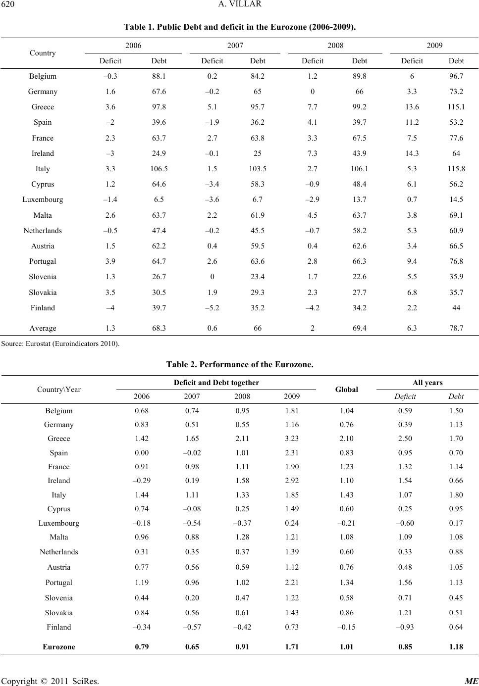

A. VILLAR 620
cit i
07 2008 2009
Table 1. Public Debt and defin the Eurozone (2006-2009).
2006 20
Country
Deficitbt Deficit Debt Debt Deficit Debt Deficit De
Belgium –0.3 88.1 0.2 84.2 1.2 89.8 6 96.7
Germany 1.6 67.6 –0.2 65 0 66 3.3 73.2
Greece 3.6 97.8 5.1 95.7 7.7 99.2 1
Luxrg
–
3.6115.1
Spain –2 39.6 –1.9 36.2 4.1 39.7 11.2 53.2
France 2.3 63.7 2.7 63.8 3.3 67.5 7.5 77.6
Ireland –3 24.9 –0.1 25 7.3 43.9 14.3 64
Italy 3.3 106.5 1.5 103.5 2.7 106.1 5.3 115.8
Cyprus 1.2 64.6 –3.4 58.3 –0.9 48.4 6.1 56.2
embou–1.4 6.5 –3.6 6.7 –2.9 13.7 0.7 14.5
Malta 2.6 63.7 2.2 61.9 4.5 63.7 3.8 69.1
Netherlands –0.5 47.4 –0.2 45.5 –0.7 58.2 5.3 60.9
Austria 1.5 62.2 0.4 59.5 0.4 62.6 3.4 66.5
Portugal 3.9 64.7 2.6 63.6 2.8 66.3 9.4 76.8
Slovenia 1.3 26.7 0 23.4 1.7 22.6 5.5 35.9
Slovakia 3.5 30.5 1.9 29.3 2.3 27.7 6.8 35.7
Finland –4 39.7 5.2 35.2 –4.2 34.2 2.2 44
Average 1.3 68.3 0.6 66 2 69.4 6.3 78.7
Source: Euroindicators 2
abl2. Pmance e Eurozone
Deficit and Debt together All years
urostat (E010).
Te erforof th.
Country\Year 2006 Global Deficit Debt
2007 2008 2009
Belgium 0.68 1.81 1.04 0.59 1.50 0.74 0.95
Germany 0.83 0.51 0.55 1.16 0.76 0.39 1.13
Greece 1.42 1.65 2.11 3.23 2.10 2.50 1.70
Spain 0.00 –0.02 1.01 2.31 0.83 0.95 0.70
France 0.
I
91 0.98 1.11 1.90 1.23 1.32 1.14
reland –0.29 0.19 1.58 2.92 1.10 1.54 0.66
Italy 1.44 1.11 1.33 1.85 1.43 1.07 1.80
Cyprus 0.74 –0.08 0.25 1.49 0.60 0.25 0.95
Luxemg –0.–0.–0.–0.–0.bour18 54 37 0.24 21 60 0.17
Malta 0.96 0.88 1.28 1.21 1.08 1.09 1.08
Netherlands 0.31 0.35 0.37 1.39 0.60 0.33 0.88
Austria 0.77 0.56 0.59 1.12 0.76 0.48 1.05
Portugal 1.19 0.96 1.02 2.21 1.34 1.56 1.13
Slovenia 0.44 0.20 0.47 1.22 0.58 0.71 0.45
Slovakia 0.84 0.56 0.61 1.43 0.86 1.21 0.51
Finland –0.34 –0.57 –0.42 0.73 –0.15 –0.93 0.64
Eurozone 0.79 0.65 0.91 1.71 1.01 0.85 1.18

A. VILLAR621
The data show that, accordinriten [6’]
there are ocountries that manda
y year 2006 and 2Luxem and
i
g to the crion i
nly two
between
eet the st
009:
rds year
bourgb
F nland. There are 7 more countries that satisfy the crite-
ria when considering the whole period: Germany, Spain,
Cyprus, Netherlands, Austria, Slovenia and Slovakia.
And there are two countries that do not meet the stan-
dards in any of the years considered: Greece and Italy.
Let us now consider whether the Stability and Growth
Pact has been fulfilled collectively along the years ana-
lyzed in Tables 1 and 2. To do so we let the weight i

of each country be given by its relative GDP. We ob-
serve that, taking the two objectives together there is
only one year in which the Eurozone did not satisfy the
criteria of the SGP (last row of Table 2). Yet the devia-
tion was bad enough as to conclude that for the whole
Eurozone and the whole period, the pact has not been
fulfilled (as

.1.01  ). Looking at each objective in-
dividually, we observe that the Eurozone has collectively
reached the deficit target (nine countries did it individu-
ally) but has ftisfy the debt target (even though
eight countries met that objective). All together the Eu-
rozone has failed to meet the standards, even though nine
of the countries have succeeded in doing it.
4.2. Research Excelence in the Spanish
Universities
ailed to sa
ellence
data re-
orted paper analyzes the performance of
ntile 8hin eachory. As weighthe
bles we re-scale those in the study that im
ollowin
We now consider the evaluation of research exc
in the Spanish public universities, out of the
in [11]. Thisp
the Spanish universities and provides an overall ranking
using a set of variables whose relative weights are deter-
mined by the opinion of researchers obtained by a spe-
cific survey. Values are relative to the size of the perma-
nent faculty in each university and are normalized so that
the top university in each dimension gets a mark of 100.6
Here we take three out of the six variables computed
by those authors, as we understand they are the most
relevant ones. These variables are: publications (in terms
of ISI papers), individual research productivity achieve-
ments, IRPA for short,7 and success in getting research
funds competitively. In order to define “excellence” we
take a relative vector of reference values given by:
175z for ISI publications, 285z for individual
productivity achievements, and 350z for research
funds. Those values correspond, approximately, to per-
ce5 wit categfor thets of
varia
f
ply the
g: 10,348


(papers), 20,328

 ),
and
(IRPA
30,324


(funds). Table 3es the data cor-
responding to the 48 Spanish univerlyzed.
The object of this exercise is to determine the set of
universities that are “excellent” from the point of view of
their research realizations in 2009.8 If we consider the
extreme valu
provid
sities ana
e



e the th
, that is, thoseities that
are abresholds in all dimensions, we find that
there are only three universities that meet those standards
of
univers
ov
excellence: Universitat Atònoma de Barcelona, Uni-
versidad Pablo de Olavide, and Universitat Pompeu
Fabra. If we take the case 0

 (the geometric mean),
we find five addiniversities entering the bonus set:
Universidad Autónoma de Madrid, Universitat de Bar-
celona, Universidad Carlos III, Universidad Miguel
Hernandez, and Universitat Rovira i Virgili. Reducing
the level of exigency to 1
tional u

 (the arithmetic mean)
does not add new universitiehat set. Finally, for the
other extreme value,
s to t


 (namely, the set of uni-
versities that satisfy at least one of those criteria), we
find that the set of excellent universities includes five
more: Alcalá, Girona, Lleida, Rey Juan Carlos, and Va-
lencia.
Table 4 gives the data of the 8 universities that meet
the excellence standard the geometric and/or the
arithmetic mean. The table contains their relative arith-
metic mean scores, information about the region in
which those universities are placed, and whe- ther they
are new (created in the last twenty years, say), modern
(c
s using
reated in the 60’s) or traditional (with a history of hun-
dreds of years). Even though discussing those data is not
the purpose of this exercise, it is quite noticeable the
success of the Catalan universities and the dominance of
new and modern universities over the traditional ones.
5. Final Comments
We have provided here a criterion to evaluate the per-
formance of a society with respect to a collection of tar-
gets. This criterion materializes in a simple an intuitive
ormula, a mean of order f

of the shares of the realiza-
h has beized by
ents. Thethe mean
tions in the targets, whic
eans of standard requirem
en character
order of m
is a parameter that determines the substitutability be-
tween the achievements and therefore the admissible
degree of compensation among the various dimensions
and the different agents. From this perspective the model
can be regarded as producing endogenously a system of
shadow prices that permits one to aggregate the different
6By “permanent Faculty” is understood here those people who are civil
servants (funcionarios) within the categories that require a doctoral
degree. That should be taken into account in order to interpret the re-
sults.
7The “tramos de investigación”, a voluntary individual research evalua-
tion carried out every six years by a central agency, that results in a
small salary increase.
8The results presented here correspond to the original figures afte
r
rounding them up to integer numbers plus at most two digits.

A. VILLAR 622
ce Table 3. Research Performanof the Spanish Universities.
Universities ISI Articles Research Bonuses Research Funds
A Coruña 19.95 65.08 25.44
Alcalá 43.72 85.71
95 80.95
36.65
Alicante 48.31.2
Autólona
Autódrid
Castilncha
Complutense Madrid
E
4
L
Las Pale G.C.
Pablo de Olavide
Politécagena
Politécnica Cataluña
Politécnica Valencia
Sa
Z
Almería 38.82 65.08 23.69
noma Barce91.88 90.47 51.12
noma Ma72.61 95.24 45.79
Barcelona 84.16 80.95 46.18
Burgos 34.99 63.49 28.68
Cádiz 30.16 66.67 19.03
Cantabria 51.53 80.95 34.6
Carlos III 62.01 100 55.53
la-La Ma57.63 77.78 36.6
27.65 77.78 32.13
Córdoba 60.51 77.78 19.53
xtremadura 39.38 77.78 19
Girona 64.91 66.67 60.68
Granada 42.92 77.78 26.94
Huelva 42.66 63.49 22.3
Islas Baleares 40.68 82.54 8.85
Jaén 56.33 66.67 38.46
Jaume I 40.5 79.36 33.06
a Laguna31.28 58.73 14.48
La Rioja 35.56 69.84 25.45
mas d19.82 50.79 17.34
León 29.86 73.01 21.99
Lleida 51.15 69.84 49.94
Málaga 30.27 69.84 20.47
Miguel Hernández 97.28 90.47 49.78
Murcia 41.51 77.78 25.67
Oviedo 37.55 76.19 23.57
80.58 92.06 62.22
País Vasco 19.23 68.25 31.44
nica Cart53.5 69.84 26.67
46.93 74.6 42.55
Politécnica Madrid 30.04 50.79 26.89
62.32 63.49 34.95
Pompeu Fabra 100 87.3 100
Pública Navarra 44.22 74.6 27.28
Rey Juan Carlos 51.48 71.43 52.43
Rovira i Virgili 90.63 84.12 46.01
Salamanca 36.58 79.36 33.77
antiago Compostel49.51 82.54 34.39
Sevilla 36.29 76.19 25.71
UNED 20.88 66.67 20.67
Valencia 55.91 87.3 30.03
Valladolid 31.52 69.84 23.22
Vigo 56.65 66.67 31.11
aragoza 46.4 79.36 29.86
Source: Buela-Cas0). al et al. (201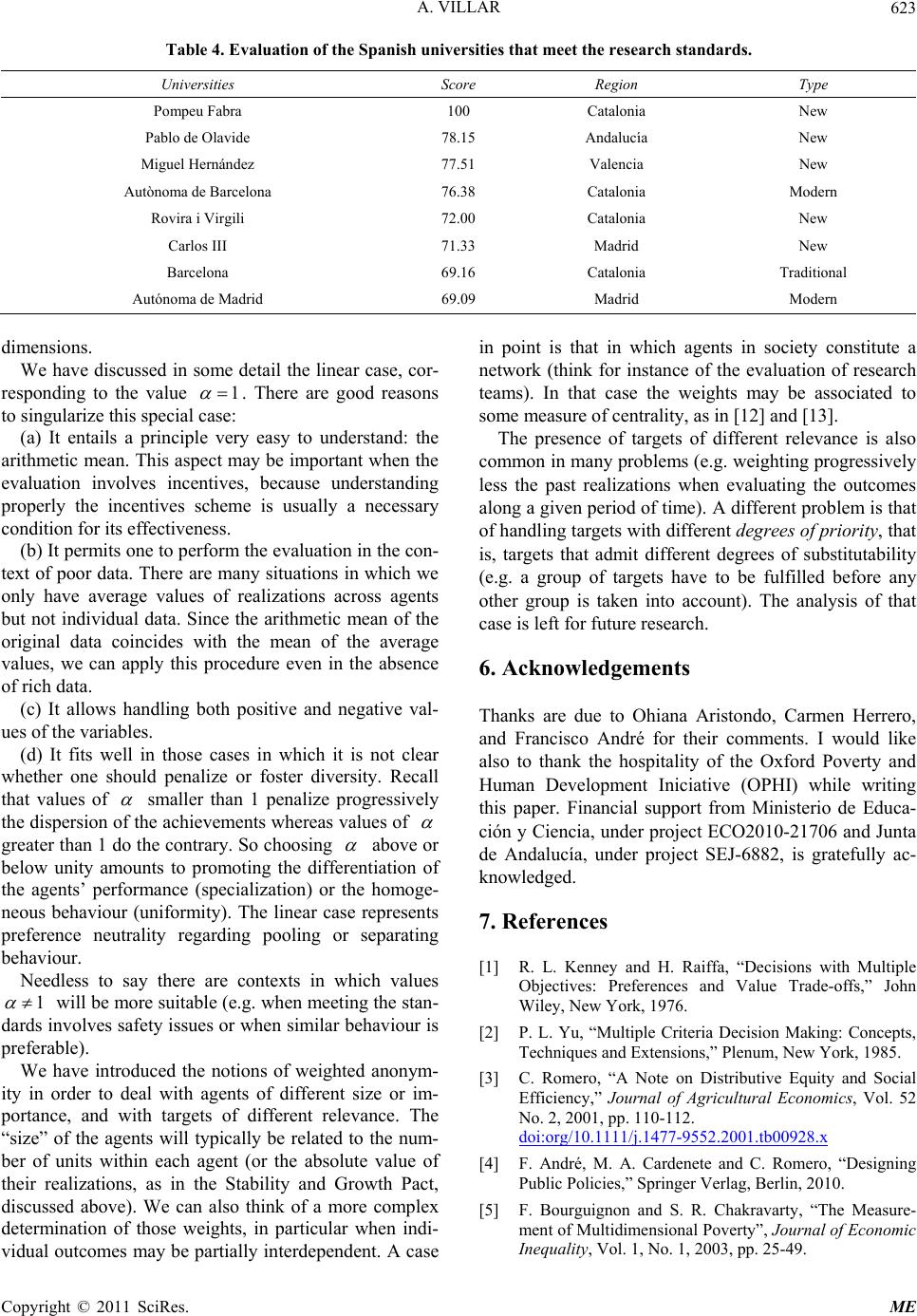

A. VILLAR623
ble 4. Evaluation of tnish universities that me research standards.
Region
Tahe Spaeet th
Universities Score Type
Pompeu Fabra 100 Catalonia New
Pablo de Olavide 78.15 Andalucía New
MiValencia
AutònoM
T
guel Hernández 77.51
76.
New
nma de Barcelona 38 Catalonia oder
Rovira i Virgili 72.00 Catalonia New
Carlos III 71.33 Madrid New
Barcelona 69.
Autónoid
16 Catalonia raditional
Mn ma de Madr69.09 Madrid oder
dimensions.
We have discussedcase, cor-
responding to th
in some detail the linear
e value 1

. There are good reasons
singularize this special case:
ls a principle very easy to understand: the
ar
ntive
is usually a necessary
co
he arithmetic mean of the
ori
hould penalize or foster diversity. Recall
th
to
(a) It entai
ithmetic mean. This aspect may be important when the
evaluation involves inces, because understanding
properly the incentives scheme
ndition for its effectiveness.
(b) It permits one to perform the evaluation in the con-
text of poor data. There are many situations in which we
only have average values of realizations across agents
but not individual data. Since t
ginal data coincides with the mean of the average
values, we can apply this procedure even in the absence
of rich data.
(c) It allows handling both positive and negative val-
ues of the variables.
(d) It fits well in those cases in which it is not clear
whether one s
at values of

smaller than 1 penalize progressively
the dispersion of the achievements whereas values of

greater than 1 do the contrary. So choosing

above or
below unity amounts to promoting the differentiation of
the agents’ perfrmance (specialization) or the homoge-
neous behaviour (uniformity). The linear case represen
preference neutrality regarding pooling or separating
behaviour.
Needless to say there are contexts in which values
1
o
ts

 will be more suitable (e.g. when meeting the stan-
dards involves safety issues or when similar behaviour is
preferable).
ity in
agents will typically be related to the num-
be
vidual outcomes may be partially interdependent. A
n point is thaich agents in society constitute a
ork (thinance of the evalesearch
ms). In thathe weights may ciated to
some measure of centrality, as in [12] and [13].
CO2010-21706 and Junta
e Andalucía, under project SEJ-6882, is gratefully ac-
,” Journal of Agricultural Economics, Vol. 52
. 110-112.
1/j.1477-9552.2001.tb00928.x
We have introduced the notions of weighted anonym-
order to deal with agents of different size or im-
portance, and with targets of different relevance. The
“size” of the
r of units within each agent (or the absolute value of
their realizations, as in the Stability and Growth Pact,
discussed above). We can also think of a more complex
determination of those weights, in particular when indi-
The presence of targets of different relevance is also
common in many problems (e.g. weighting progressively
less the past realizations when evaluating the outcomes
along a given period of time). A different problem is that
of handling targets with different degrees of priority, that
is, targets that admit different degrees of substitutability
(e.g. a group of targets have to be fulfilled before any
other group is taken into account). The analysis of that
case is left for future research.
case
it in wh
netwk for instuation of r
teat case be asso
6. Acknowledgements
Thanks are due to Ohiana Aristondo, Carmen Herrero,
and Francisco André for their comments. I would like
also to thank the hospitality of the Oxford Poverty and
Human Development Iniciative (OPHI) while writing
this paper. Financial support from Ministerio de Educa-
ción y Ciencia, under project E
d
knowledged.
7. References
[1] R. L. Kenney and H. Raiffa, “Decisions with Multiple
Objectives: Preferences and Value Trade-offs,” John
Wiley, New York, 1976.
[2] P. L. Yu, “Multiple Criteria Decision Making: Concepts,
Techniques and Extensions,” Plenum, New York, 1985.
[3] C. Romero, “A Note on Distributive Equity and Social
Efficiency
No. 2, 2001, pp
doi:org/10.111
. Chakravarty, “The Measure-
[4] F. André, M. A. Cardenete and C. Romero, “Designing
Public Policies,” Springer Verlag, Berlin, 2010.
[5] F. Bourguignon and S. R
ment of Multidimensional Poverty”, Journal of Economic
Inequality, Vol. 1, No. 1, 2003, pp. 25-49.

A. VILLAR 624
doi:org/10.1023/A:1023913831342
[6] S. R. Chakravarty, “A Generalized Human Development
Index”, Review of Development Economics, Vol. 7, No. 1,
2003, pp. 99-114. doi:org/10.1111/1467-9361.00178
ultidimen-
e
[7] C. Herrero, R. Martinez and A. Villar, “M
sional Social Evaluation. An Application to the Measure-
ment of Human Development”, The Review of Incom
and Wealth, Vol. 56, No. 3, 2010, pp. 483-497.
doi:org/10.1111/j.1475-4991.2009.00375.x
[8] S. Seth, “A Class of Sensitive Multidimen
Indices,” Vanderbilt University, Nashv
sional Welfare
ille, Mimeo 2010.
[9] K. Tsui, “Multidimensional Poverty Indices,” Social
Choice and Welfare, Vol. 19, No. 1, 2002, pp. 69-93.
doi:org/10.1007/s355-002-8326-3
[10] A. Villar, “A New Approach to the Measurement of Mul-
tidimensional Poverty,” Pablo de Olavide University
a,
. (2010), Ranking de
l and Y. Zenou, “Who's
Working Paper, Seville, 2010.
[11] G. Buela-Casal, M. P. Bermúdez and J. C. Sierr
“Quevedo-Blasco, R. & Castro, A
2009 en Investigación de las Universidades Públicas
Españolas,” Psicothema, Vol. 22, pp. 171-179.
[12] C. Ballester, A. Calvó-Armengo
Who in Networks. Wanted: the Key Player,” Economet-
rica, Vol. 74, No. 5, 2006, pp. 1403-1417.
doi:org/10.1111/j.1468-0262.2006.00709.x
[13] B. Ruhnau, “Eigenvector-centrality: A Node Centrality?”
Social Networks, Vol. 22, No. 4, 2000, pp. 357-365.
doi:org/10.1016/S0378-8733(00)00031-9