Modern Economy, 2011, 2, 602-613
doi:10.4236/me.2011.24068 Published Online September 2011 (http://www.SciRP.org/journal/me)
Child Benefit and Fiscal Burden: OLG Model with
Endogenous Fertility
Kazumasa Oguro, Junichiro Takahata, Manabu Shimasawa
Associate Professor, Hitotsubashi University, Tokyo, Japan
Research Associate, JICA Research Institute, Tokyo, Japan.
Associate Professor, Akita University, Akita, Japan
Received May 31, 2011; revised July 12, 2011; accepted July 22, 2011
Abstract
In this paper, we present an OLG simulation model with endogenous fertility to analyze the relationship be-
tween child benefit and fiscal burden. Our simulation results show that expansion of the child benefit will
improve the welfare of current and future generations. On the other hand, our findings show that we cannot
expect a significant long-term improvement in welfare solely from the increase of the consumption tax. If
both the fiscal sustainability and the improvement of the welfare of current and future generations are re-
quirements, we will need a policy-mix that includes both child benefit expansion and additional fiscal re-
form.
Keywords: Computable General Equilibrium (CGE) Model, Overlapping Generations (OLG), Child Benefit,
Endogenous Fertility
1. Introduction
Developed countries currently face unprecedented demo-
graphic changes which require extensive reform in fiscal
systems, social security systems, and other related pro-
grams. However, due to conflicting interests between
younger and older generations, reform may be restricted.
As an example of a pay-as-you-go pension, in order to
improve the sustainability of the system, the government
has the option of reducing the benefits to the elderly or
increasing the burden on the working generation. Ob-
taining agreement on reform by both generations is often
too difficult for the government to achieve. In this situa-
tion, some developed countries such as France have pro-
ceeded with the expansion of child benefit programs.
These programs are expected to increase the population
of the younger generation as a tax resource and, as result,
to reduce the per capita fiscal burden in the future.
In this paper we analyze the relationship between child
benefit and the fiscal burden in the setting of an overlap-
ping generations (OLG) model. In the process of this
analysis, it is important for us to distinguish between an
exogenous fertility model and an endogenous fertility
model. The reason is that recent studies have clarified
that the Pareto-efficiency condition of the exogenous
fertility model differs from that of the endogenous fer-
tility model. First, for an exogenous fertility model, we
use the OLG model introduced by Diamond [1]. Three
types of steady states exist in the model: under-accumu-
lation, golden rule, and over-accumulation. The first two
steady states are Pareto-efficient, but the third is not. In
addition, an empirical study by Abel et al. [2] reports
that in industrialized countries dynamic efficiency is sa-
tisfied. In a steady state, dynamic efficiency corresponds
to under-accumulation (or golden rule). Therefore, the
possibility that developed countries are in a state of un-
der-accumulation seems high. In an exogenous fertility
setting, an allocation is said to be Pareto-efficient if it is
impossible to make some individuals better off without
making other individuals worse off. For this reason, in an
exogenous case, we cannot improve any generation’s
utility while at the same time sacrificing another gene-
ration’s utility.
However, recent studies clarify the properties of the
competitive equilibrium with an endogenous fertility set-
ting. Raut and Srinivasan [3] and Charkrabarti [4] analyze
the properties of intertemporal equilibrium with endoge-
nous fertility. Conde-Ruiz et al. [5] and Golosov et al. [6]
present the definition of Pareto-efficiency criteria in an
endogenous fertility framework.

K. OGURO ET AL.603
As a development of these studies, Michel and Wig-
niolle [7]1 point out the possibility that under-accumu-
lation may not be efficient in an endogenous fertility set-
ting. This implies that some policies could effect impro-
vement in one generation’s welfare without sacrificing
another generation’s welfare, even when it is in an under-
accumulation state near the steady state. Moreover, the
remarkable point made by Michel and Wigniolle [7] is to
clarify that the Representative-Consumer efficient (RC-
efficient) condition, which is a concept developed in their
study, has a profound connection with the sign-of-inequa-
lity relationship between the child-rearing cost and wage
rate.2 That is, if some policies do provide effects to this
relationship, improvement in RC-efficiency becomes
possible. Michel and Wigniolle [7] provide proof that, by
utilizing an OLG model with endogenous population
growth, the possibility to improve RC-efficiency also
exists in the case of under-accumulation. But they did not
analyze an economy model with public debt. Therefore,
Oguro and Takahata [13] analyze the relationship be-
tween child benefit and fiscal burden, in the setting of an
OLG model with both endogenous fertility and public
debt, and provide the condition of RC-efficiency. How-
ever, they also could not analyze the relationship between
child benefit and fiscal burden in a real economy. The
reason is that the overlapping generations of their OLG
model amount to only two: the working generation and
the retired generation. To analyze the relationship in a
real economy, it is necessary to build an OLG model with
more overlapping generations: e.g., a model with 85 over-
lapping generations and endogenous fertility.
To this end, we construct a large-scale numerical dyna-
mic equilibrium OLG model with endogenous fertility,
which is calibrated to the Japanese economy. And we
quantitatively evaluate the effects of child benefit change:
e.g., the effects on the welfare of multiple generations. By
doing this, we attempt to answer whether a fundamental
change in child benefit policy results in significant posi-
tive effects on the Japanese economy, especially in terms
of the government fiscal situation.
The structure of this paper is as follows. In Section 2,
we describe the model structure; Section 3 presents the
calibration strategy and the findings; Section 4 describes
simulation results, and Section 5 contains concluding
remarks and policy implications.
2. The Model Structure
In this section, we describe the demographic and econo-
mic structure of our model. The model used here is a
computable general-equilibrium OLG model with perfect
foresight agents, multiple periods, and endogenous fertil-
ity. In our model, there is a representative individual for
each generation in the households sector. Each individual
at age 20 maximizes his/her intertemporal utility function
with consumption and number of children. The repre-
sentative competitive firm has a standard Cobb-Douglas
production technology and maximizes its profits. In our
model, not only the goods market but also factor markets
are perfectly competitive. The model has five main
building blocks: 1) household behavior, 2) firm behavior,
3) the Government, 4) the public pension, and 5) market
equilibrium. Details of each block follow.
2.1. Household Behavior
There is a representative individual for each generation
in the household sector. We assume that preferences
forms are the same for all agents in all generations.
Moreover, each individual lives for a fixed number of
periods. In each period of the model, the oldest genera-
tion dies and a new one enters. And the representative
individuals maximize their intertemporal utility function
with consumption and number of their children subject to
their lifetime income. They are also assumed to be ra-
tional, having perfect foresight. Each generation enters
the labor market at age 21, bears and brings up their
children at ages 21 to M + 20, retires at age 1Q

, is
granted a pension at , and dies at age
Q
Z
. In addition,
each supplies labor inelastically. The within-period util-
ity function exhibits constant relative risk aversion, and
preferences are additive and separable over time. In each
region, the utility functions of the t th generation born in
year t are specified as:3

2
11
120 ,
1
12
1
1
11
j
Ztj
t
tj
c
n
U



1






 



(1)
where

refers to the weight between number of chil-
dren and consumption, 1

the preference parameter of
number of children, j the j th period of life,

the pure
rate of time preference, and 2

the reverse of the elas-
ticity of intertemporal substitution of consumption. The
arguments of the utility function are the number of chil-
dren (t) and the consumption per period (,tj
). Leisure
does not enter the utility function since the individual’s
labor supply is assumed to be exogenous.
nc
1Although there have been several approaches that endogenize fertility
decisions, Michel and Wigniolle [7] depend on the benchmark frame-
work, which assumes that children are consumption goods that appear
in the utility function of the parents. The basic articles are Becker [8],
Willis [9], and Eckstein and Wolpin [10]. Other approaches depend on
the literature based on the additional assumption of descendant altruism
as in Becker and Barro [11] or the assumption of ascendant altruism
and strategic behavior of parents, as in Nishimura and Zhang [12].
2The definition of “RC-efficiency” can be seen in Michel and Wig-
niolle [7] or Oguro and Takahata [13].
3This is the expansion of the utility function provided by Groezen et al.
[14]. If σ1 = σ2 = 1 and Z = 22, i.e. only two periods (working period
and retired period), this utility function becomes the same form as that
of Groezen et al. [14].

K. OGURO ET AL. 604

In addition, we assume that the number of children
(,tj n) whom the t th generation bears at the j th period of
life is the following:
 
 
,
where0if 120
and0 if20
tjj t
j
j
npn
pjM
pjM



(2)
where


11tr R

refers to the factor of the present
discounted value which is driven from the gross interest
rate t and the capital tax t tr in year t, R
g

is the
child rearing cost at the g th period of life, t

is the
government subsidy in year t, t is the consumption
tax rate in year t, t is the labor income tax rate in
year t, t
tc
tw
w

is the public pension contribution rate in year
t, t is the net lifetime income of generation t, t is
the wage rate in year t, t
NW w
p

is the tax for pension bene-
fit in year t, and t stands for pension benefit in year t.
In addition, child rearing cost is assumed to be propor-
tional to net lifetime income, i.e.,
q
g
g
NWt

 , where
where
j
p refers to the possibility that each generation
bears the children at the j th period of life and this pa-
rameter is assumed to be exogenous.
Moreover, the technological progress

is assumed
to be exogenous and labor embodied. We model age-
specific labor productivity by assuming a hump-shaped
age-earnings profile, i.e., a quadratic form of its age j, so
its age-wage profile
j
e takes the following form:
g

is the constant parameter.
Each generation maximizes its utility function (1) un-
der the budget constraint (4).
2
01 2
01 2
, 0 and 0
j
ej  
 
 

j
(3)
The intertemporal budget equation of each generation
is described as follows:




120 , 20 20
1 11
20 20
1
20 , 20
1
20 20
1
20
21 2020 20
1
20 20
1
20
1
1
1
1
(1)(1 )
(1 )
(1 )
gtjgtj M
jg jg
tk tk
k
tj tj Z
t
j
j
tk tk
k
tj
Qtjtj tjj
j
j
tk tk
k
tj tj
n
tr R
tc cNW
tr R
tww we
tr R
pq



 
 
 

 

 


 

 

 





 







20 20
20
20 20
1(1 )
Z
j
jQ
tk tk
ktr R


 


(4)
When 12




nc
, the maximization procedure dif-
ferentiating the household utility function (2) with re-
spect to t and ,tj
, subject to the individual’s lifetime
budget constraint (4), yields the following equations
concerning consumption per period and number of chil-
dren.



1/
20
,
20 20
1
1
1
111
jtj
tj j
tk tk
k
tc
ctr R




 
















,


1/
120 20 20
1 11
20 20
1
1
1
gtjg j
M
tjg
jg
tk tk
k
p
ntr R





 
 














,
(5)
and





/
1/ 20
1/
1/ 11/ 1 1
120 20 20 20
1 11
20 2020 20
11
1
11
11
11
j
Z
t
j
gtjg jtj M
jg j jg
tk tktk tk
kk
NW
ptc
tr RtrR











 



  

 
  

 



 

 



 

 



 








If the parameter

is stable, these equations dictate
the following two relationships: 1) as in any life-cycle
model, the trade-off between current and future con-
sumption is determined by the ratio of the interest rate
and the time preference rate, and by the degree of risk
aversion, and 2) the number of children declines, when
the child rearing cost increases or the government sub-
sidy decreases. Moreover, from these equations, the fol-
lowing forms can be shown:
20 20
20, 20,
11
,
ZM
tttjjt ttj
jj
CNcN Nn

 



j
(6)
where is the aggregated consumption in year t, and
t measures the number of the generation born in year t.
In addition, we can also derive the following physical
wealth accumulation equation:
t
C
N





 
,,1 120 120
2020 ,
20 ,20,1
1
20
20,
1
1
1
1 1
and
tj tjtj tj
tjtj tj
j
tj tjgtjtjg
g
Z
tttjj
j
aa trR
tww w
tc cn
PANa



 
 





 
 



,
(7)
where ,tj is physical wealth asset of generation t at the
j th period of life, and is the aggregated private
a
t
PA

K. OGURO ET AL.605
0
N
asset in year t.
2.2. Firm behavior
The input/output structure is represented by the Cobb-
Douglas production function with constant return to scale.
The firm decides the demand for physical capital and
effective labor in order to maximize its profit with the
given factor prices of wage and rent, which are deter-
mined in the perfect competitive markets.

1
,
20
,2
11
ttet
t
Q
etjtj
j
YAKL
Le








, (8)

1
1
tt t
K
I 

 K (9)
where t is output, Y

stands for capital income share,
A is a scale parameter, t
K
is the physical capital stock,
and is the effective labor.
,et
We can derive two factor prices, the rate of return rt
and the wage rate per unit of effective labor wt, by the
first-order conditions for the firm’s maximum profit:
L


11
,
,
11
1
tt tet
ttet
RrAKL
wAKL







  
 (10)
where

is the depreciation of physical capital.
2.3. The public pension
The pension sector grants a pension to the retirement
generations while pension contribution is collected from
the working generations.
,ttt
PwwL
et

 (11)
where stands for the aggregated pension contribu-
tion.
t
P
The aggregated pension benefits in year t is given by
the product of the population of retirement age, replace-
ment rate, and average earnings of each generation dur-
ing the working period t
W.
20 20
20 2020 20
19 19
ZZ
t tjtjtjtj
jQ jQ
BqN WN 

  
 

(12)
where

denotes replacement rate and is the ag-
gregated pension benefit.
t
B
We explicitly model the public pension system as pay-
as-you-go. The budget constraint of the pension sector
can be shown as follows:


1
t
Psp t B (13)
where
s
pdenotes public subsidy to pension, which is
financed by government expenditure .
t
Moreover, we assume that the public pension sector
maintains a fixed replacement rate exogenously. As a
result, in our model, the pension contribution rate is en-
dogenously determined in order to keep the budget con-
straint (13).
G
2.4. The Government
The government sector has four types of taxes: wage tax,
consumption tax, capital tax, and pension benefit tax, and
the public debt issue income as its revenue and pays the
consumption, investment, and interest payments as ex-
penditures.
,tttettttttt
TtwwL tcCtrRPAtpB
t

 (14)
We keep all tax rates constant. The role of the gov-
ernment is to endogenously determine the rate of the
public debt issue as a residual of government expenditure
and revenue.

1
1
ttt tt
DGT rD

 (15)
where t stands for government expenditure in year t,
t denotes tax revenue in year t, denotes public
debt in year t.
G
Tt
D
The public debt issue

1
1
tt tt
BondDr D

 is set
endogenously due to the difference between expenditure
and tax revenue. It should be noted that the public debt
issue to GDP ratio will change over time as a result of
possible imbalances between revenues and expenditures.
Thus we don’t know whether the fiscal policy of a coun-
try is sustainable and whether the government’s in-
tertemporal budget constraint must be satisfied.
2.5. Market Equilibrium
Finally, in our model of a closed economy, we require
the equilibrium in the financial market, i.e., the aggregate
value of assets equals the market value of the capital
stocks plus the value of outstanding government bonds:
tt
PA KD
t
(16)
3. The Data, Calibration, and Scenarios
3.1. Data and Calibration
First, we present the values of the main parameters and
exogenous variables of the model in Table 1. The pa-
rameter values for the households’ and firms’ behaviors
are derived from Auerbach and Kotlikoff [15] and vari-
ous early OLG simulation studies in Japan.4 These pa-
rameters, such as technological and preference parame-
ters except the weight parameter

, are assumed to be
constant.
4See Sadahiro and Shimasawa [16,17]; Uemura [18]; and Ihori et al.
[19].

K. OGURO ET AL. 606
Table 1. Parameter Values of the Model.
PARAMETER VALUE
Utility function
Time preference rate

0.01
Intertemporal elasticity of substitution 1

2.0
Weight parameter between children number and consumption

0.84*
Production function
Technology progress

0.002
Capital share in production

0.3
Physical capital depreciation

0.05
Tax policy parameters
Wage tax tw 20.0%
Capital tax tr 20.0%
Consumption tax tc 5.0%
Pension benefit tax tp 10.0%
Pension policy parameters
National subsidy to pension
s
p 25.0%
Replacement ratio

50.0%
Other parameters
0 to 5 0.78%
6 to 10 0.46%
11 to 15 0.55%
Child rearing cost to net lifetime income
16 to 20 0.58%
1 to 5 3.0%
6 to 10 7.4%
11 to 15 7.0%
Child bearing possibility
16 to 20 2.6%
Government subsidy to child rearing cost

0.1
Limit age of bearing child
M
40
Age of retirement Q 65
Average life expectancy
Z
85
* This parameter is fixed after year 2007.
The exogenous variables such as the macroeconomic,
fiscal, and public pension variables are derived mainly
from OECD [20] “Tax Database,” and Whitehouse [21]
“Pensions Panorama.”
In addition, the child bearing possibility parameter is
derived from the data of “Age-specific fertility rate,”
which is provided by the National Institute of Population
and Social Security Research [22], and the parameter
values of the child rearing cost and the government sub-
sidy are derived from the special research report about
social cost of rearing children, which is provided by the
Cabinet Office Director-General for Policies on a Cohe-
sive Society, Japan [23].
Second, by controlling the weight parameters in years
1900 - 2007, we calibrate our demographic projection to
fit the data’s trend in “Population by Age (generation
born in 1900 - 2007),” which is provided by the Statistics
Bureau, Ministry of Internal Affairs and Communica-
tions with the collaboration of other Ministries and
Agencies in Japan. Figure 1 reports the actual values and
the computed values of demographic projection. Note
that actual and calculated values correspond closely.
Next, in order to analyze the relationship between
child benefit and fiscal burden, we start our calculations

K. OGURO ET AL. 607
Figure 1. Demographic Projection of Each Generation.
with a phase-in period of about 200 years in order to re-
lax the unrealistic assumption of a steady state in the
2007 base year of our simulation. Moreover, since the
model is simulated over 500 periods, we ensure a suffi-
ciently long period for a steady state to be achieved.
Table 2 reports the actual values of some key variables
in 2007 and the computed values in the model. Also,
note that actual and calculated values correspond closely.
3.2. Scenarios
Next we present simulation scenarios (See Table 3). The
scenarios are classified into four categories. Scenario 1
assumes the baseline case with no expansion of child
benefit, and Scenarios 2 and 3 assume 100% increase of
child benefit after 2015. Scenario 4 assumes 50% in-
crease of child benefit after 2015. Scenarios 5 and 6 as-
sume no expansion of child benefit but an increase in the
consumption tax to 10% and 15% (consumption tax re-
form), respectively. Finally, Scenario 7 is the policy-mix
of Scenario 2 (permanent expansion) and Scenario 6
(15% consumption tax reform).
In Scenarios 2 and 4, the increase of child benefit is
permanent from 2015. In Scenario 3, the increase of
child benefit is temporal for 2015-2025.
4. Simulation Results
We now turn to describe the simulation results reported
in Figures 2 to 5 and Table 4. Here we present the sce-
narios of results of the child benefit expansion in com-
parison to the cases of no expansion, the case of con-
sumption tax reform, and the case of policy-mix (per-
manent expansion and consumption tax reform).
4.1. Demographic Projection and
Macroeconomic Variables
Figure 2 shows the population projection of future gen-
erations born in 2000 - 2030. The projection of Scenario
1 and official estimation, which is provided by the Na-
tional Institute of Population and Social Security Re-
search [23], closely correspond. In Scenario 2 (100%
permanent child benefit increase), compared with Sce-
nario 1, the population of the generation born in 2030
increases by 143,000, in Scenario 3 (100% temporally
child benefit increase) by 11,000, in Scenario 4 (50%
permanent child benefit increase) by 66,000, in Scenario
5 (10% consumption tax reform) by –4,000, in Scenario
6 (15% consumption tax reform) by 19,000, and in Sce-
nario 7 (policy-mix) by 166,000.5
Figure 3 also shows the retired population ratio. The
ratio of Scenario 1 and official estimation, which is pro-
vided by the National Institute of Population and Social
5Consumption tax reform may contribute to the increase of population
of future generations through the mechanism in that the fall in net life-
time income decreases the child rearing cost, e.g., the opportunity cost
which is the net lost income when parents bring up a child.

K. OGURO ET AL. 608
Table 2. Year 2007 of the Baseline Scenario.
OFFICIAL MODEL
National Inco me (% of GDP)
Private consumption 74.1% 81.3%
Government purchases of goods and services 21.0% 24.3%
Saving rate 3.1% 6.1%
Government Indicators
Pension premium to wage 14.9% 14.9%
Gross public debt (% of GDP) 170.6% 170.6%
Primary balance (% of GDP) –2.4% –4.5%
Tax revenues (% of GDP) 18.4% 19.8%
Other Indicators
Capital output ratio 2.9 4.6
Interest rate 1.7% 2.6%
Data source: Official values are derived from OECD Economic Outlook No. 84, 2008 and “Annual Report on National Accounts,” the Japanese SNA statistics
(Cabinet Office).
Table 3. Scenarios.
Scenario 1 Scenario 2 Scenario 3 Scenario 4 Scenario 5 Scenario 6 Scenario 7
Child benefit No increase 100% increase after
2015
100% increase for
2015 - 25
50% increase after
2015 No increase No increase 100% increase
after 2015
Consumption tax 5% 5% 5% 5% 10% 15% 15%
Figure 2. Simulation Results－Demographic Projection of Future Generation.

K. OGURO ET AL.609
Table 4. Simulation Results－Macro Economic Projection.
GDP
GDP per
employee
Saving
rate
Capital-
labor ratio
Interest
rate Wage rateDebt-GD P ratio
Debt per
employee
Pension
premium
to wage
Scenario 1 2007 100.00%100.00% 6.17% 100.00%2.61% 100.00%170.65% 100.00% 14.90%
2010 98.63% 101.30% 5.59% 101.82%2.51% 100.54%186.94% 108.02% 15.83%
2015 94.49% 104.03% 5.82% 104.68%2.37% 101.38%219.79% 123.21% 17.37%
2020 90.34% 106.21% 0.69% 105.60%2.32% 101.65%259.60% 141.98% 25.99%
2030 80.75% 103.92% 1.16% 95.61% 2.85% 98.66% 364.40% 192.97% 26.45%
Scenario 2 2007 100.00%100.00% 6.17% 100.00%2.61% 100.00%170.79% 100.00% 14.90%
2010 98.63% 101.30% 5.59% 101.82%2.51% 100.54%187.15% 108.06% 15.83%
2015 94.51% 104.05% 6.06% 104.74%2.36% 101.40%220.38% 123.46% 17.37%
2020 90.33% 106.20% 0.95% 105.57%2.32% 101.64%261.87% 142.96% 25.99%
2030 80.66% 103.81% 1.49% 95.27% 2.87% 98.56% 371.39% 194.48% 26.48%
Scenario 3 2007 100.00%100.00% 6.17% 100.00%2.61% 100.00%170.77% 100.00% 14.90%
2010 98.63% 101.30% 5.59% 101.82% 2.51% 100.54%187.12% 108.05% 15.83%
2015 94.49% 104.03% 6.05% 104.69%2.37% 101.39%220.33% 123.43% 17.37%
2020 90.31% 106.18% 0.93% 105.52%2.33% 101.63%261.71% 142.97% 25.99%
2030 80.67% 103.82% 1.24% 95.30% 2.87% 98.57% 369.45% 195.11% 26.48%
Scenario 4 2007 100.00%100.00% 6.17% 100.00%2.61% 100.00%170.72% 100.00% 14.90%
2010 98.63% 101.30% 5.59% 101.82%2.51% 100.54%187.05% 108.04% 15.83%
2015 94.50% 104.04% 5.94% 104.71%2.37% 101.39%220.08% 123.33% 17.37%
2020 90.33% 106.20% 0.81% 105.58%2.32% 101.64%260.70% 142.45% 25.99%
2030 80.71% 103.87% 1.31% 95.45% 2.86% 98.61% 367.70% 193.71% 26.46%
Scenario 5 2007 100.00%100.00% 6.17% 100.00%2.61% 100.00%170.49% 100.00% 14.90%
2010 98.63% 101.30% 5.59% 101.82% 2.51% 100.54%186.71% 107.98% 15.83%
2015 92.39% 101.72% 6.86% 97.14% 2.76% 99.13% 222.73% 122.20% 17.37%
2020 89.40% 105.10% –0.43% 101.98%2.50% 100.59%246.94% 133.75% 26.38%
2030 81.08% 104.35% –2.02% 96.93% 2.78% 99.07% 305.60% 162.55% 26.65%
Scenario 6 2007 100.00%100.00% 6.17% 100.00%2.61% 100.00%170.38% 100.00% 14.90%
2010 98.63% 101.30% 5.59% 101.82%2.51% 100.54%186.51% 107.95% 15.83%
2015 90.47% 99.60% 7.84% 90.56% 3.15% 97.07% 225.78% 121.38% 17.37%
2020 88.56% 104.12% –1.65% 98.84% 2.67% 99.65% 235.22% 126.26% 26.74%
2030 81.28% 104.60% –5.45% 97.71% 2.73% 99.31% 251.16% 133.71% 26.89%
Scenario 7 2007 100.00%100.00% 6.17% 100.00%2.61% 100.00%170.51% 100.00% 14.90%
2010 98.63% 101.30% 5.59% 101.82%2.51% 100.54%186.73% 107.99% 15.83%
2015 90.49% 99.63% 8.14% 90.63% 3.15% 97.09% 226.46% 121.67% 17.37%
2020 88.55% 104.11% –1.31% 98.80% 2.67% 99.64% 237.98% 127.50% 26.74%
2030 81.19% 104.49% –4.99% 97.37% 2.75% 99.20% 259.50% 136.54% 26.92%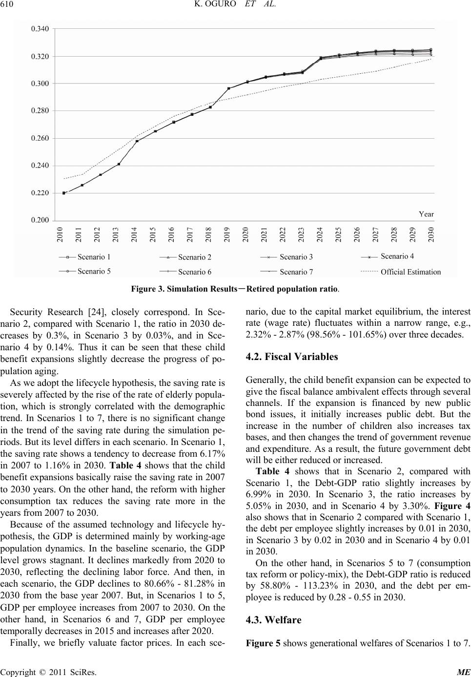

K. OGURO ET AL. 610
Figure 3. Simulation Results－Retired population ratio.
nario, due to the capital market equilibrium, the interest
rate (wage rate) fluctuates within a narrow range, e.g.,
2.32% - 2.87% (98.56% - 101.65%) over three decades.
Security Research [24], closely correspond. In Sce-
nario 2, compared with Scenario 1, the ratio in 2030 de-
creases by 0.3%, in Scenario 3 by 0.03%, and in Sce-
nario 4 by 0.14%. Thus it can be seen that these child
benefit expansions slightly decrease the progress of po-
pulation aging.
4.2. Fiscal Variables
Generally, the child benefit expansion can be expected to
give the fiscal balance ambivalent effects through several
channels. If the expansion is financed by new public
bond issues, it initially increases public debt. But the
increase in the number of children also increases tax
bases, and then changes the trend of government revenue
and expenditure. As a result, the future government debt
will be either reduced or increased.
As we adopt the lifecycle hypothesis, the saving rate is
severely affected by the rise of the rate of elderly popula-
tion, which is strongly correlated with the demographic
trend. In Scenarios 1 to 7, there is no significant change
in the trend of the saving rate during the simulation pe-
riods. But its level differs in each scenario. In Scenario 1,
the saving rate shows a tendency to decrease from 6.17%
in 2007 to 1.16% in 2030. Table 4 shows that the child
benefit expansions basically raise the saving rate in 2007
to 2030 years. On the other hand, the reform with higher
consumption tax reduces the saving rate more in the
years from 2007 to 2030.
Table 4 shows that in Scenario 2, compared with
Scenario 1, the Debt-GDP ratio slightly increases by
6.99% in 2030. In Scenario 3, the ratio increases by
5.05% in 2030, and in Scenario 4 by 3.30%. Figure 4
also shows that in Scenario 2 compared with Scenario 1,
the debt per employee slightly increases by 0.01 in 2030,
in Scenario 3 by 0.02 in 2030 and in Scenario 4 by 0.01
in 2030.
Because of the assumed technology and lifecycle hy-
pothesis, the GDP is determined mainly by working-age
population dynamics. In the baseline scenario, the GDP
level grows stagnant. It declines markedly from 2020 to
2030, reflecting the declining labor force. And then, in
each scenario, the GDP declines to 80.66% - 81.28% in
2030 from the base year 2007. But, in Scenarios 1 to 5,
GDP per employee increases from 2007 to 2030. On the
other hand, in Scenarios 6 and 7, GDP per employee
temporally decreases in 2015 and increases after 2020.
On the other hand, in Scenarios 5 to 7 (consumption
tax reform or policy-mix), the Debt-GDP ratio is reduced
by 58.80% - 113.23% in 2030, and the debt per em-
ployee is reduced by 0.28 - 0.55 in 2030.
4.3. Welfare
Finally, we briefly valuate factor prices. In each sce- Figure 5 shows generational welfares of Scenarios 1 to 7.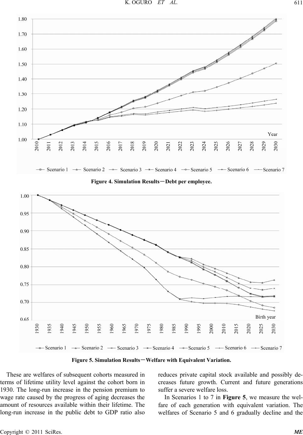

K. OGURO ET AL. 611
Figure 4. Simulation Results－Debt per employee.
Figure 5. Simulation Results－Welfare with Equivalent Variation.
These are welfares of subsequent cohorts measured in
terms of lifetime utility level against the cohort born in
1930. The long-run increase in the pension premium to
wage rate caused by the progress of aging decreases the
amount of resources available within their lifetime. The
long-run increase in the public debt to GDP ratio also
reduces private capital stock available and possibly de-
creases future growth. Current and future generations
suffer a severe welfare loss.
In Scenarios 1 to 7 in Figure 5, we measure the wel-
fare of each generation with equivalent variation. The
welfares of Scenario 5 and 6 gradually decline and the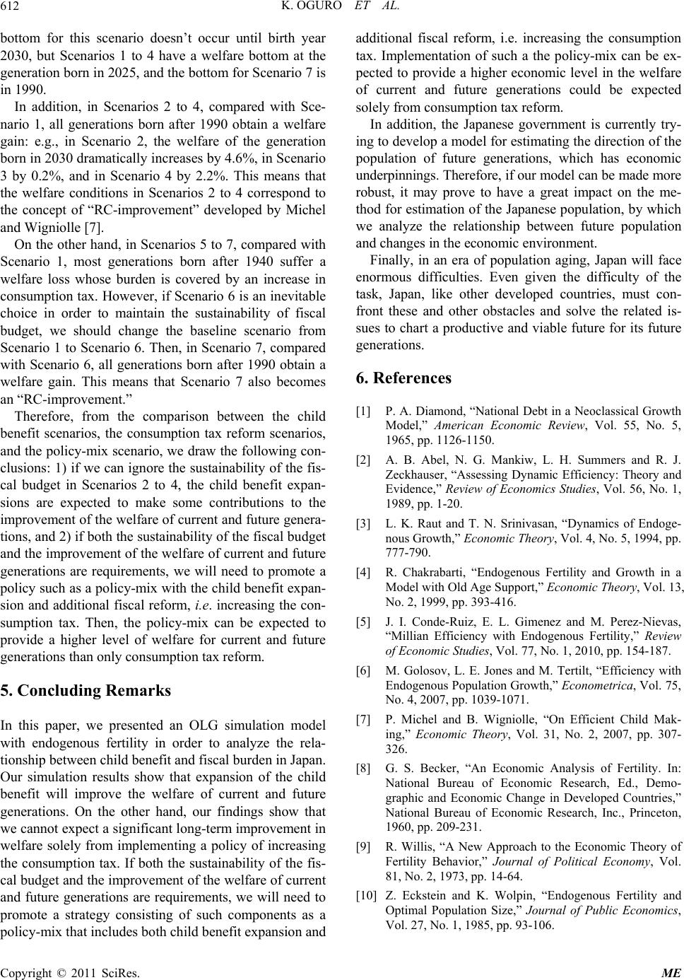

K. OGURO ET AL. 612
bottom for this scenario doesn’t occur until birth year
2030, but Scenarios 1 to 4 have a welfare bottom at the
generation born in 2025, and the bottom for Scenario 7 is
in 1990.
In addition, in Scenarios 2 to 4, compared with Sce-
nario 1, all generations born after 1990 obtain a welfare
gain: e.g., in Scenario 2, the welfare of the generation
born in 2030 dramatically increases by 4.6%, in Scenario
3 by 0.2%, and in Scenario 4 by 2.2%. This means that
the welfare conditions in Scenarios 2 to 4 correspond to
the concept of “RC-improvement” developed by Michel
and Wigniolle [7].
On the other hand, in Scenarios 5 to 7, compared with
Scenario 1, most generations born after 1940 suffer a
welfare loss whose burden is covered by an increase in
consumption tax. However, if Scenario 6 is an inevitable
choice in order to maintain the sustainability of fiscal
budget, we should change the baseline scenario from
Scenario 1 to Scenario 6. Then, in Scenario 7, compared
with Scenario 6, all generations born after 1990 obtain a
welfare gain. This means that Scenario 7 also becomes
an “RC-improvement.”
Therefore, from the comparison between the child
benefit scenarios, the consumption tax reform scenarios,
and the policy-mix scenario, we draw the following con-
clusions: 1) if we can ignore the sustainability of the fis-
cal budget in Scenarios 2 to 4, the child benefit expan-
sions are expected to make some contributions to the
improvement of the welfare of current and future genera-
tions, and 2) if both the sustainability of the fiscal budget
and the improvement of the welfare of current and future
generations are requirements, we will need to promote a
policy such as a policy-mix with the child benefit expan-
sion and additional fiscal reform, i.e. increasing the con-
sumption tax. Then, the policy-mix can be expected to
provide a higher level of welfare for current and future
generations than only consumption tax reform.
5. Concluding Remarks
In this paper, we presented an OLG simulation model
with endogenous fertility in order to analyze the rela-
tionship between child benefit and fiscal burden in Japan.
Our simulation results show that expansion of the child
benefit will improve the welfare of current and future
generations. On the other hand, our findings show that
we cannot expect a significant long-term improvement in
welfare solely from implementing a policy of increasing
the consumption tax. If both the sustainability of the fis-
cal budget and the improvement of the welfare of current
and future generations are requirements, we will need to
promote a strategy consisting of such components as a
policy-mix that includes both child benefit expansion and
additional fiscal reform, i.e. increasing the consumption
tax. Implementation of such a the policy-mix can be ex-
pected to provide a higher economic level in the welfare
of current and future generations could be expected
solely from consumption tax reform.
In addition, the Japanese government is currently try-
ing to develop a model for estimating the direction of the
population of future generations, which has economic
underpinnings. Therefore, if our model can be made more
robust, it may prove to have a great impact on the me-
thod for estimation of the Japanese population, by which
we analyze the relationship between future population
and changes in the economic environment.
Finally, in an era of population aging, Japan will face
enormous difficulties. Even given the difficulty of the
task, Japan, like other developed countries, must con-
front these and other obstacles and solve the related is-
sues to chart a productive and viable future for its future
generations.
6. References
[1] P. A. Diamond, “National Debt in a Neoclassical Growth
Model,” American Economic Review, Vol. 55, No. 5,
1965, pp. 1126-1150.
[2] A. B. Abel, N. G. Mankiw, L. H. Summers and R. J.
Zeckhauser, “Assessing Dynamic Efficiency: Theory and
Evidence,” Review of Economics Studies, Vol. 56, No. 1,
1989, pp. 1-20.
[3] L. K. Raut and T. N. Srinivasan, “Dynamics of Endoge-
nous Growth,” Economic Theory, Vol. 4, No. 5, 1994, pp.
777-790.
[4] R. Chakrabarti, “Endogenous Fertility and Growth in a
Model with Old Age Support,” Economic Theory, Vol. 13,
No. 2, 1999, pp. 393-416.
[5] J. I. Conde-Ruiz, E. L. Gimenez and M. Perez-Nievas,
“Millian Efficiency with Endogenous Fertility,” Review
of Economic Studies, Vol. 77, No. 1, 2010, pp. 154-187.
[6] M. Golosov, L. E. Jones and M. Tertilt, “Efficiency with
Endogenous Population Growth,” Econometrica, Vol. 75,
No. 4, 2007, pp. 1039-1071.
[7] P. Michel and B. Wigniolle, “On Efficient Child Mak-
ing,” Economic Theory, Vol. 31, No. 2, 2007, pp. 307-
326.
[8] G. S. Becker, “An Economic Analysis of Fertility. In:
National Bureau of Economic Research, Ed., Demo-
graphic and Economic Change in Developed Countries,”
National Bureau of Economic Research, Inc., Princeton,
1960, pp. 209-231.
[9] R. Willis, “A New Approach to the Economic Theory of
Fertility Behavior,” Journal of Political Economy, Vol.
81, No. 2, 1973, pp. 14-64.
[10] Z. Eckstein and K. Wolpin, “Endogenous Fertility and
Optimal Population Size,” Journal of Public Economics,
Vol. 27, No. 1, 1985, pp. 93-106.

K. OGURO ET AL. 613
[11] G. S. Becker and R. J. Barro, “A Reformulation of the
Economic Theory of Fertility,” Quarterly Journal of
Economics, Vol. 103, No. 1, 1988, pp. 1-25.
[12] K. Nishimura, and J. Zhang, “Pay-As-You-Go Public
Pensions with Endogenous Fertility,” Journal of Public
Economics, Vol. 48, No. 2, 1992, pp. 239-258.
[13] K. Oguro and J. Takahata, “Child Benefit and Fiscal
Burden with Endogenous Fertility,” Discussion Papers on
Demography and Policy, No. 2009-001, 2009, Public
Economics Program, School of International and Public
Policy, Hitotsubashi University.
[14] B. V. Groezen, T. Leers and L. Meijdam, “Social Secu-
rity and Endogenous Fertility: Pensions and Child Al-
lowances as Siamese Twins,” Journal of Public Econom-
ics, Vol. 87, No. 2, 2003, pp. 233-251.
[15] A. J. Auerbach and L. J. Kotlikoff, “Dynamic Fiscal Pol-
icy,” Cambridge University Press, Cambridge, 1987.
[16] A. Sadahiro and M. Shimasawa, “Fiscal Sustainability
and the Primary Surplus: A Simulation Analysis with
OLG Model,” JCER Economic Journal, Vol. 43, No. 2,
2001, pp.117-132.
[17] A. Sadahiro and M. Shimasawa, “The Computable Over-
lapping Generations Model with an Endogenous Growth
Mechanism,” Economic Modeling, Vol. 20, No. 1, 2003,
pp. 1-24.
[18] T. Uemura, “Lifecycle General Equilibrium Analysis on
Social Security,” Keizaironshu, Vol. 28, No. 1, 2002, pp.
15-36.
[19] T. Ihori, R. Kato, M. Kawade and S. Bessho, “Public
Debt and Economic Growth in an Aging Japan. In: Kai-
zuka, K. and Krueger, A. O. Ed.,” Tackling Japan’s Fis-
cal Challenges: Strategies to Cope with High Public Debt
and Population Aging, Palgrave Macmillan, New York,
2006, pp. 30-68.
[20] OECD Tax Database, 2007.
http://www.oecd.org/document/60/0,3746,en_2649_3453
3_1942460_1_1_1_1,00.html
[21] Whitehouse, “E. Pensions Panorama: Retirement-Income
Systems in 53 Countries,” World Bank, Washington D.
C., 2007.
[22] National Institute of Population and Social Security Re-
search Population Statistics of Japan, 2007.
http://www.ipss.go.jp/syoushika/tohkei/Popular/Popular2
007.asp?chap=0
[23] Cabinet Office Director-General for Policies on a Cohe-
sive Society, Japan, Shakai Zentai no Kosodate Hiyo ni
kansuru Chosa Kenkyu Hokokusho, 2005.
http://www8.cao.go.jp/shoushi/cyousa/cyousa16/kosodate
/index_pdf.html
[24] National Institute of Population and Social Security Re-
search, Population Projections for Japan: 2006-2055.
2006.
http://www.ipss.go.jp/syoushika/tohkei/suikei07/index.asp