Applied Mathematics, 2011, 2, 1182-1190
doi:10.4236/am.2011.29164 Published Online September 2011 (http://www.SciRP.org/journal/am)
Multi-Team Bertrand Game with Heterogeneous Players
Mohammed Fathy Elettreby1*, Daoud Suleiman Mashat2, Ashraf Mobarez Zenkour2
1Mathematics Department, Facu lty of Science, King Khaled University, Abha, Saudi Arabia
2Department of Mat hem at i cs, Faculty of Science , King Abdulaziz University, Jeddah, Saudi Arabia
Received March 9, 2011; revised June 8, 2011; accepted June 15, 2011
Abstract
In this paper, we proposed a general form of a multi-team Bertrand game. Then, we studied a two-team Ber-
trand game, each team consists of two firms, with heterogeneous strategies among teams and homogeneous
strategies among players. We find the equilibrium solutions and the conditions of their local stability. Nume-
rical simulations were used to illustrate the complex behaviour of the proposed model, such as period dou-
bling bifurcation and chaos. Finally, we used the feedback control method to control the model.
Keywords: Bertrand Game, Non-Convex Dynamical Multi-Team Game, Incomplete Information Dynamical
System, Marginal Profit Method, Nash Equilibrium
1. Introduction
Game theory [1,2] is the study of multi-person decision
problem. Such problems arise in economics. The game is
called incomplete information if at least one of the
players does not know the other player's payoff, such as
in an auction when the bidders do not know the offers of
each other. Otherwise, it is called complete information
game. Also, the game can be classified to static or dyna-
mic game. There are two famous economic games, the
first is the Cournot game [3] and the second is the
Bertrand game [4]. In economic games, the first step is to
construct the game. The second step is to solve the game
(get their Nash equilibrium) and study the stability of
these equilibria. Nash [5] showed that in any finite game
there exists at least one Nash equilibrium.
Nature push us to make teams in all fields. This has at
least two main advantages. The first is the improvement
of our profit and the second is that living in a team
reduces the risk. For example, in the forest animals live
in teams (herds). Since looking for food in a team is
more efficient than doing it alone and reduces predation
risk due to early spotting of predators and that existing in
a team gives a higher probability that the predator will
attack another member of the team. Another example is
the competition between firms in the market. Suppose
M
branches of McDonald fast food shops compete
against branches of Kentucky fast food shops.
N
Multi-team game has been studied in [6]. In their work,
they proposed and applied the concept of multi-team
game in the hock-dove game, prisoner dilemma game
and Cournot game. Also, the Cournot multi-team game
has been studied in [7-11]. The standard static Bertrand
game has been studied in [12]. A duopoly Bertrand game
with bounded rationality is studied in [13]. Multi-team
bertrand game is studied in [14] with two teams but the
second team consists of one player.
We will construct the model in Section 2. In Section 3,
we will analysis the model, i.e., we will find its equi-
librium points and their stability conditions. Some nume-
rical analysis will be done in Section 4 to show the com-
plexity behaviour of the model. Finally in section 5, we
will use the feedback control method to control our
odel.
m
2. The Model
Bertrand game is a model of competition used in eco-
nomics. It describes interaction among firms that set
prices and their customers that choose quantities at that
price. In this game there are at least two firms producing
homogeneous products and compete by setting prices
simultaneously. Consumers buy everything from a firm
with a lower price. If all firms have the same price,
consumers randomly select among them.
Suppose there are totally firms (produce certain
product) in the market and these firms are divided into
teams. Let ij be the price per unit of that product
produced by the firm in the team and let ij c be
the marginal cost of producing one unit of that product
n
Npj i

M. F. ELETTREBY ET AL.1183

by the firm in the team . Then, the payoff of the
firm in the team , if it played without the team, is
given by the following equations;
j
=
ij
i

1,,
a
i
ji
,
pc

π=,
1,, =,
ij ijijlkij
i
bppp
iNjN

(1)
where is the number of teams and i is the
number of firms in the team . The positive constants
are the demand parameters where is the slop of
the demand function.
N N
,ab b
We propose that, firms in the same team share some of
their payoffs with their team mates. So, let i
lj

be the
payoff rate that firm will takes from the payoff of
firm in the same team . It is clear that ,
j
i
lj

=1
12
12
l
i
lj
i0<  <1
i
lj
<1 
l
of the first firm of the first team , if he
played with the team, is given by the followimg;
and . For example, the final payoff <1
j

j

=1i

π
i

11 1
131 11
1
11 1
21311 1
11
=1 π
π,
N
NN
 
 


11
13
ππ

lj
where 1 is the number of firms in the first team. In
general, the final payoff of the firm in the team i is
given by;
Nj
=1 π
NN
ii
i
ijjlijlj il
lj



 




(2)
In the case of two teams


=2N
=2
where each team
consists of two firms and from Equation
(1), we get the following payoffs of the firms in each
team;

12
=NN

11
=
=
=
b
b
b
b





,
,
.




12
21
22



1111 11122122
12121211 21 22
2121212211 12
22222221 11 12
=,
pca p p pp
pcapppp
pcapp pp
pcapppp




π
π
π
π
(3)
Using the assumption in Equation (2) of sharing some
of the payoffs and Equation (3), we get the final payoffs
of the firms as follows:





11
11121121 12
11
12211212 11
22
21122121 22
22
22212212 21
=1 ππ,
=1 ππ,
=1 ππ,
=1 ππ.




 
 
 
 
(4)
In this model, we assume that the firms in the first
team use the marginal profit method [15], to expect their
profit for the next time according to the following
equations;

1
1
1111
1
=,
tj
tt t
jjjj
tj
pp pj
p


=1,2,
(5)
where 1
j

is the speed (rate) of adjustment and it is a
function of the price 1
j
p. The firms in the second team
use Nash equilibrium [2], to make their decision for the
next step by solving the following equations;
2
2
=0, =1,2.
tj
tj
j
p

 (6)
In this model, we assume that the speed of adjustment
will be linear and take the form

11 11
=
tt
j
jj
pp 
j
, and
1>0 j

. Substituting from Equation (4) in Equations (5)
and (6), we get the following system (7);
Then, Equation (7) describe a system of two teams,
each team consists of two firms with homogeneous
strategies among each firms in each team and heteroge-
eous strategies among teams. n
3. The Analysis of the Model
The steady state (equilibrium) solutions are very interest
[16]. In the context of difference equations, an
equilibrium solution
x
is defined to be the value that
satisfies the relations 1==
tt
x
xx
. Then, we can get
the equilibrium solutions for our model by the following.
Let

 


 



11 1
11
12
1
21
22
t
p




111112111112212221 1212
11 1
121221121211 21 22121111
2
21
22111222 22
2
12
=1 2,
=1 2,
1
=,
221
tt tttttt
tt tttttt
ttttt
ppabcbpppp pc
ppabcbpppp pc
cppp pc
bb
 
 


11
12
21
p
p
bpa










 





2
12
21 11 122121
2
21
1
=.
221
tttt
abpppp c
bb




1
22
c
(7)

M. F. ELETTREBY ET AL. 1184
,
.
11
11 1111121212
11
212121 222222
==,==
==,==
tt tt
tt tt
pppppp
pppppp


(8)
Then, using Equation (8), the equilibrium points are
given by solving the following system:
 


 





11
11 11121111122122211212
11
1212211212 11 21 22121111
2
21
212122111222 22
2
12
2
12
222221 11 1221
2
21
12
12
1
=,
221
1
=221
t
t
pabcbpppppc
pabcbpppppc
pabcppp pc
bb
pabcpppp
bb
 
 





 


 






21 .c
=0,
=0,
(9)
We get three boundary equilibrium solution points and
the fourth one is the coexistence equilibrium one. The
first boundary equilibrium one is given by
12
1
11
=0,0, ,,
ll
Edd



where







22 222 22
11221211212
=4 1111,db   
21


 







 
222222222222
121 121221211221121221222112
=12112 11111,labc bcb    

2
21



 







 


2222 22222222
21221211221122112 222112212112
=1211112 111.la bcbcb    
2
The second boundary equilibrium one is given by 12
212
22
=0,,,,
nn
Ep
dd



where
 










2
122 22222
221122112212112
=1411112 1212 12,db bbbb   













 

 

 

222 11
121 122121121121
12222 22
21 211221121221
12222 2
2121 22211221
=2 11211 211
21411112 12
2114112 12,
nbba bcbc
bcbbb b
bcbbbb
 

 
 
 
  
1
12














 
 
 
 

 

222 11
212211221121121
12222 2
211221122112
12222 22
21 221221212112
=2 11211 211
2114112 12
2141111212.
nbbabcbc
bcbbbb
bcbbb b
 
 

 
 
 
1
12

and


1
12 21212 11
12 1
221
=.
221
abc dnnc
pbd b




The third boundary equilibrium one is given by
12
311
33
=,0,,
mm
Ep
dd



, where
 










2
122 22222
312122112212112
=1411112121212db bbb  b 











 

 

 




222 11
121 122112121121
12222 22
12 211221121221
12222 2
1221 22211221
=2 11211211
21411112 12
2114112 12,
mbba bbcc
bcbbb b
bcbbbb
 

 

  
  
1
12



M. F. ELETTREBY ET AL.1185












 

 

 




222 11
212211212121121
122222
1212 21122112
1222222
12 221221212112
=2 112112(1)1
2114112 12
21411112 12.
mbba bbcc
bcbbbb
bcbbb b
 


 
  
  
1
12


and


1
11 31221 12
11 1
312
=.
221
abcdmmc
pbd b




The most important one is the coexistence one


4444
411122122
=,,,Epppp,where










 

43113443 123443213443223443
4
11
43 34
21111 221121 22 121122 122122 1 4
12
21 12
431134431234432134 43 4
21
2
= ,
2
= ,
2
=
aBBcDBFBcEBHBcFBDBcHBEB
pAB AB
aBBcDBFBcEBHBcFBDBcHBEB
pAB AB
aAAcDAFAcEAHAcFADA
p
 

 

 

  
22 3443
43 34
21111221121221 211221 221221 4
12
21 12
,
2
= ,
cHAEA
BA BA
aAA cDAFAcEAHA cFADA cHAEA
pBA BA


 

where,













 

1
21 11111
122112 2112 21
111
1221 12
3
21 11111
122112 2112 21
111
2112 21
2
22 22222
122112 2112 21
222
1221 12
=
81 1211,
1121
=
81 1211,
(1) 121
=
81 1211,
(1) 121
A
b
b
A
b
b
B
b
b
B
 

 

 

 

 

 







4
22 22222
122112 2112 21
222
2112 21
=
81 1211,
1121
b
b
 

 


  


 
2
11 1111
12211212 2121
111
1221 12
=
41 211211
,
1121
A
b
b
 

 








4
11 1111
12211212 2121
111
2112 21
=
41 211211
,
1121
A
b
b
 

 


 






  


 
1
22 2222
12211212 2121
222
1221 12
3
22 2222
12211212 2121
222
211221
=
41 211211
,
1121
=
41 211211
,
1121
B
b
b
B
b
b
 

 

 

 
















 

11
12 21
111
21 12
211111
12211221 12
3111
2112 21
22
12 21
222
21 12
2222 22
12211221 12
4222
2112 21
21
=,
12 (1)
4112 1
=,
1121
21
=,
12 1
4112 1
=,
1121
b
Db
b
Db
b
Db
b
Db


























11
12 21
311
12 21
2111 11
12212112 21
1111
1221 12
21
=,
12 1
4112 1
=,
1121
b
Eb
b
Eb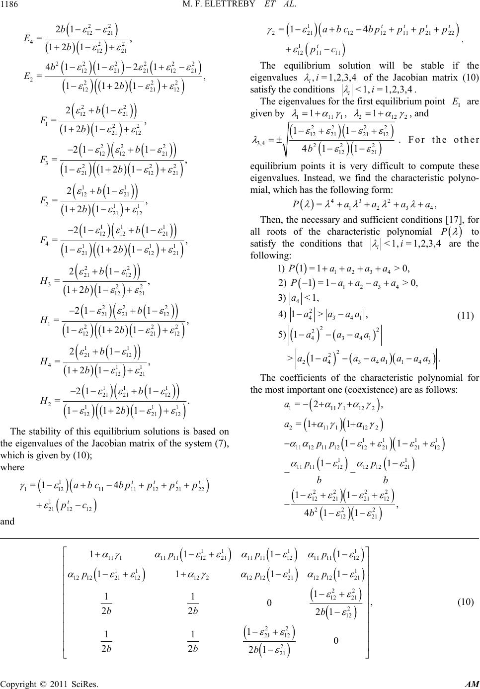









M. F. ELETTREBY ET AL. 1186










22
12 21
422
12 21
2222 22
12212112 21
2222
1221 12
21
=,
12 1
4112 1
=
1121
b
Eb
b
Eb







,
 


 









  









22
12 21
122
21 12
22 2
12 1221
322
2112 21
11
12 21
211
21 12
11 1
12 1221
411
2112 21
22
21 12
322
12 21
2
21 21
1
21
=,
12 1
21 1
=
2
1
11 21
21
=,
12 1
21 1
=,
1121
21
=,
12 1
21
=
b
Fb
b
Fb
b
Fb
b
Fb
b
Hb
H


 



 






 



 




 


 
,
 


  




22
12
222
1221 12
11
21 12
411
12 21
11 1
21 2112
2111
1221 12
1
,
1121
21
=,
12 1
21 1
=.
1121
b
b
b
Hb
b
Hb




 





 

The stability of this equilibrium solutions is based on
the eigenvalues of the Jacobian matrix of the system (7),
which is given by (10);
where





1
112 11111221
1
21 1212
=14 tt tt
t
abcbp p pp
pc




22
and





1
2211212112122
1
12 11 11
=14 tttt
t
abcbpppp
pc



 .
The equilibrium solution will be stable if the
eigenvalues , =1,2,3,4
ii

of the Jacobian matrix (10)
satisfy the conditions <1, =1,2,3,4
ii
 .
The eigenvalues for the first equilibrium point are
given by
1
E
111
11




, 212 12



 , and



22 22
12212112
3,4 22 2
12 21
11
41 1b



 
  . For the other
equilibrium points it is very difficult to compute these
eigenvalues. Instead, we find the characteristic polyno-
mial, which has the following form:


432
123
=,Paaa    
4
a
Then, the necessary and sufficient conditions [17], for
all roots of the characteristic polynomial


P

to
satisfy the conditions that <1, =1,2,3,4
ii
 are the
following:







1234
1234
4
2
4341
22
2
4341
2
2
24 341143
1)1= 1>0,
2) 1=1>0,
3)< 1,
4) 1>,
5) 1
>1
Paaaa
Paaaa
a
aaaa
aaaa
aa aaaaaa




 .
(11)
The coefficients of the characteristic polynomial for
the most important one (coexistence) are as follows:


 






1111122
2111122
11 11
11 1211 1212212112
11
11 1112121221
22 22
12212112
22 2
12 21
=2 ,
=1 1
11
11
11
,
411
a
a
pp
pp
bb
b
 
 



 






 

 





 




11 11
1111111 12211111 12 1111 12
111 1
12 12211212212 122112 1221
22
12 21
2
12
22
21 12
2
21
111
11 11
1
11 ,
0
22 21
1
11 0
22
21
ppp
pp
bb b
bb
b
   
 








 













1
p

(10)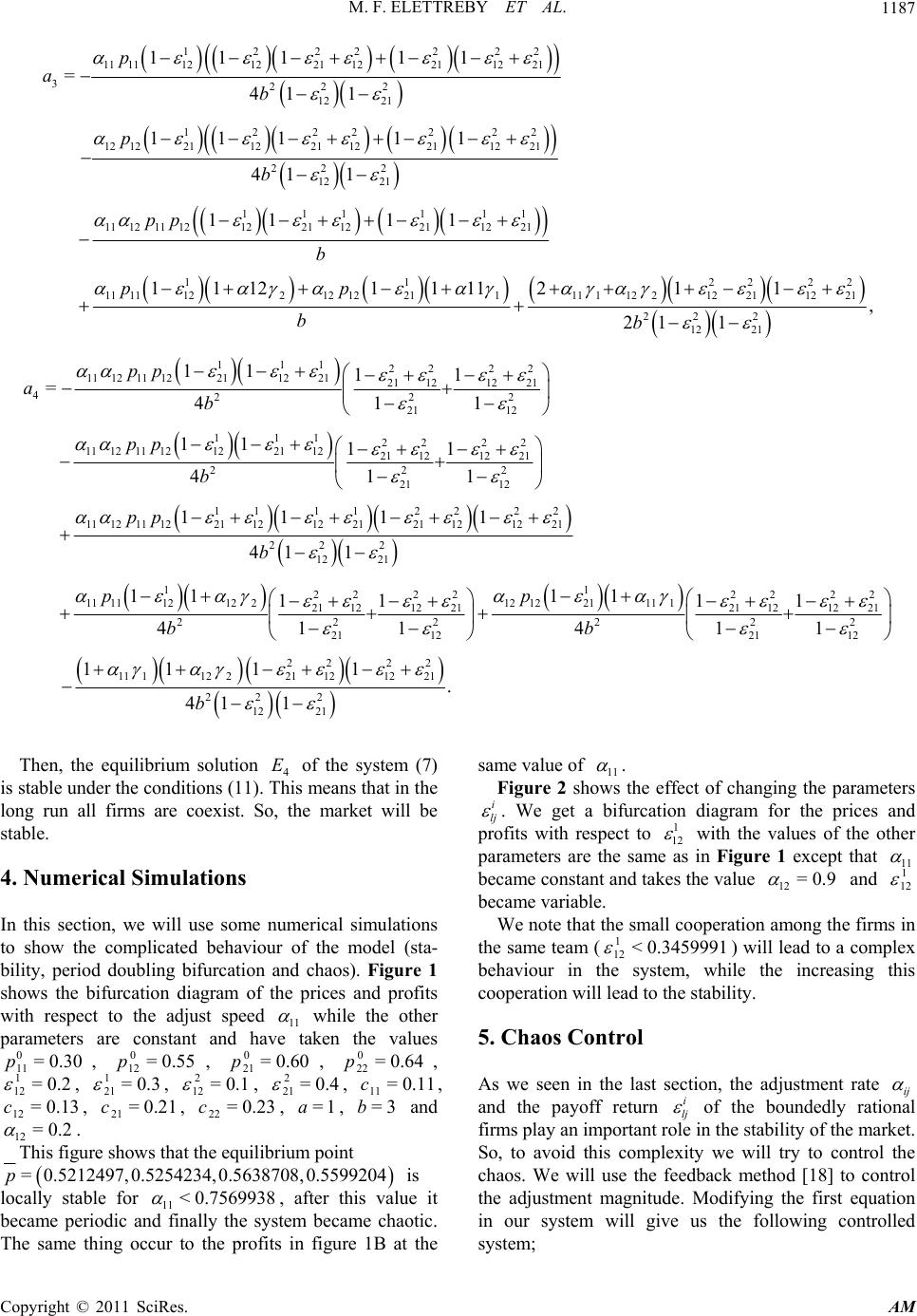

M. F. ELETTREBY ET AL.1187












 
  

 

 
1222222
11 1112122112211221
322 2
12 21
1222 222
12 1221122112211221
22 2
12 21
1111 11
11 1211 12122112211221
1
11 11122
111 11
=41 1
111 11
41 1
1111
1112
p
ab
p
b
pp
b
p




 







 

  

12
121221111112212211221
22 2
12 21
1111211 ,
21 1
p
bb
 

 

222




 

11122 22
11 12 11 1221122121121221
4222
21 12
111 2222
11 12 11 1212211221121221
222
21 12
11 1122
1112111221 12122121 12
11 11
=411
11 11
411
1111
pp
ab
pp
b
pp


 

   


 






 




   


 
   
  

22
12 21
222
12 21
1 1
22 2222 22
11 1112122121221111
21 12122121 121221
22222
21 1221 12
22 22
11 112221121221
22
12
41 1
11 11
11 11
411 411
11 11
411
b
pp
bb
b


 
2

 
 
  



 
 
  

 
 
 
 






2
21
.
Then, the equilibrium solution 4 of the system (7)
is stable under the conditions (11). This means that in the
long run all firms are coexist. So, the market will be
stable.
E
4. Numerical Simulations
In this section, we will use some numerical simulations
to show the complicated behaviour of the model (sta-
bility, period doubling bifurcation and chaos). Figure 1
shows the bifurcation diagram of the prices and profits
with respect to the adjust speed 11

while the other
parameters are constant and have taken the values
, , , ,
, , , , ,
, , , , and
0
11 =0.30p
1
12 =0.2

12 =0.13c
12 =0.2
0
12 =0.55p
1
21 =0.3 2 12

21 =0.21 c
0
21
p
=0.1 =0
=0.2
=0.60
2
21

3a
0
22 =0.64p
411 =0.1c
=3b

c. =1
1
22

.
This figure shows that the equilibrium point

= 0.5212497,0.5254234,0.5638708,0.5599204p

is
locally stable for 11 < 0.7569938

, after this value it
became periodic and finally the system became chaotic.
The same thing occur to the profits in figure 1B at the
same value of 11

.
Figure 2 shows the effect of changing the parameters
i
lj

. We get a bifurcation diagram for the prices and
profits with respect to 1
12

with the values of the other
parameters are the same as in Figure 1 except that 11

became constant and takes the value 12 =0.9

and 1
12

became variable.
We note that the small cooperation among the firms in
the same team () will lead to a complex
behaviour in the system, while the increasing this
ooperation will lead to the stability.
1
12
 < 0.3459991
c
5. Chaos Control
As we seen in the last section, the adjustment rate ij

and the payoff return i
lj

of the boundedly rational
firms play an important role in the stability of the market.
So, to avoid this complexity we will try to control the
chaos. We will use the feedback method [18] to control
the adjustment magnitude. Modifying the first equation
in our system will give us the following controlled
system;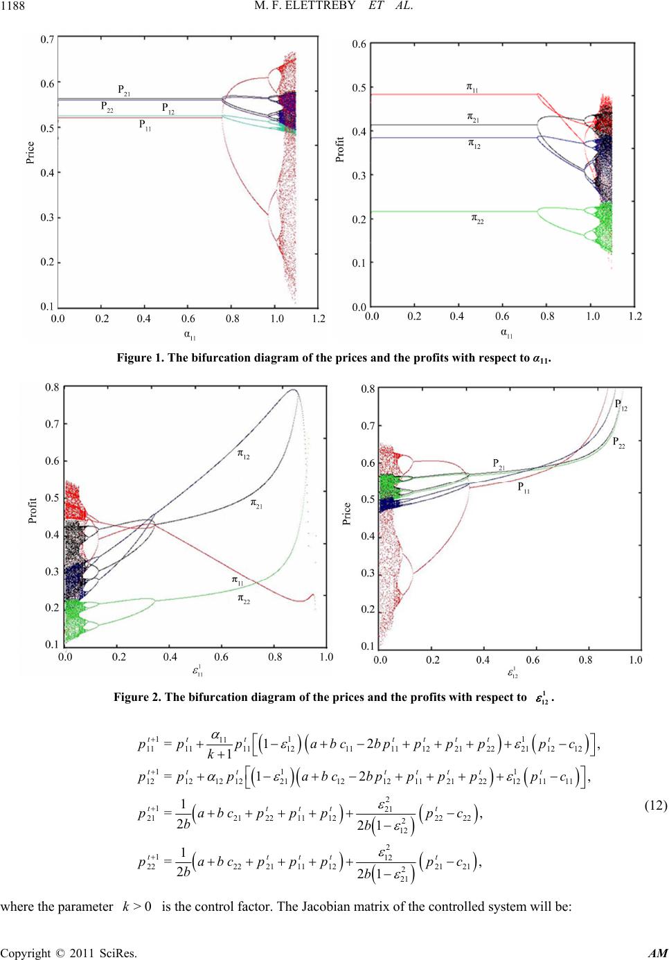

M. F. ELETTREBY ET AL. 1188
Figure 1. The bifurcation diagram of the prices and the profits with respect to α11.
Figure 2. The bifurcation diagram of the prices and the profits with respect to 1
12

.
 
 



11 1
11
11111112111112212221 1212
11 1
12121212211212 11 21 22121111
2
121
212122111222 22
2
12
2
=1 2
1
=1 2
1
=,
221
tt tttttt
tt tttttt
ttttt
pp pabcbpppppc
k
pp pabcbpppppc
pabcppppc
bb
p

 














,
,



2
112
222 2111122121
2
21
1
=,
221
ttttt
abcpppp c
bb


 

(12)
where the parameter is the control factor. The Jacobian matrix of the controlled system will be: >0k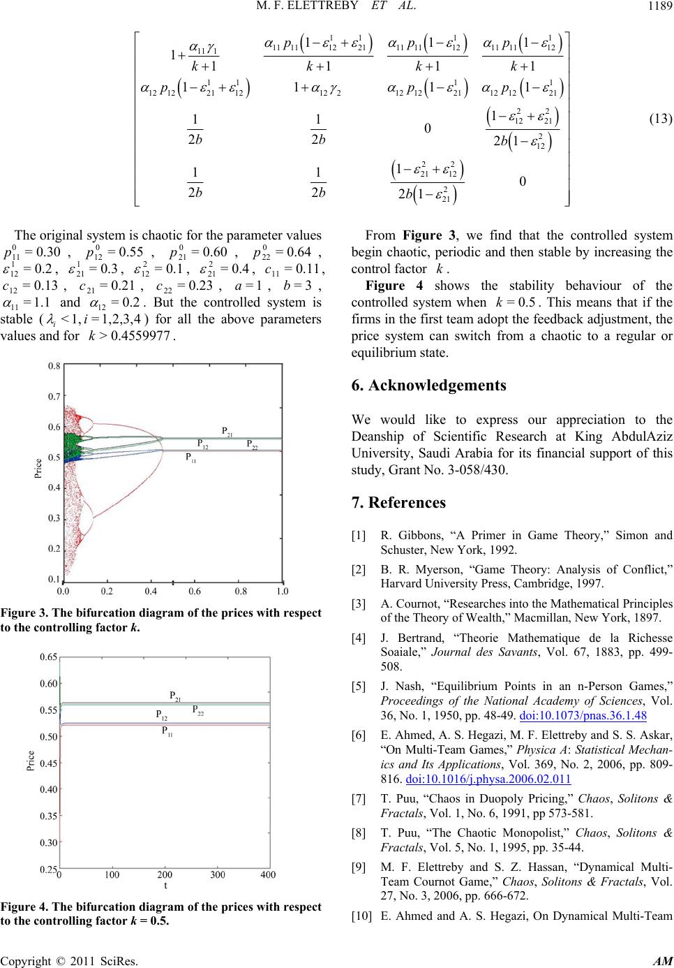

M. F. ELETTREBY ET AL.1189






 





1111
11 11122111 111211 1112
11 1
111 1
12 12211212212 1221121221
22
12 21
2
12
22
21 12
2
21
11
1111
11 1
1
11
0
22 21
1
11 0
22
21
ppp
kkkk
pp
bb b
bb
b


 





  




 














1
1
1p

(13)
The original system is chaotic for the parameter values
, , , ,
, , , , 11,
, 21 , 22 , , ,
11
0
11 =0.30p
1
12 =0.2

12 =0.13c
=1.1
0
12 =0.55p
1
21 =0.3 2 12

=0.21c
0
21 =0.60p
=0.1 2
21 =0

=0.23
0
22 =0.64p
4=0.1c
=1 =3b
 .
a1 c

and 12 =0.2

. But the controlled system is
stable (i<1, =1,2,3,4i

) for all the above parameters
values and for . > 0.455k9977
Figure 3. The bifurcation diagram of the prices with respect
to the controlling factor k.
Figure 4. The bifurcation diagram of the prices with respect
to the controlling factor k = 0.5.
From Figure 3, we find that the controlled system
begin chaotic, periodic and then stable by increasing the
control factor . k
Figure 4 shows the stability behaviour of the
controlled system when . This means that if the
firms in the first team adopt the feedback adjustment, the
price system can switch from a chaotic to a regular or
equilibrium state.
= 0.5k
6
. Acknowledgements
We would like to express our appreciation to the
Deanship of Scientific Research at King AbdulAziz
University, Saudi Arabia for its financial support of this
study, Grant No. 3-058/430.
7. References
[1] R. Gibbons, “A Primer in Game Theory,” Simon and
Schuster, New York, 1992.
[2] B. R. Myerson, “Game Theory: Analysis of Conflict,”
Harvard University Press, Cambridge, 1997.
[3] A. Cournot, “Researches into the Mathematical Principles
of the Theory of Wealth,” Macmillan, New York, 1897.
[4] J. Bertrand, “Theorie Mathematique de la Richesse
Soaiale,” Journal des Savants, Vol. 67, 1883, pp. 499-
508.
[5] J. Nash, “Equilibrium Points in an n-Person Games,”
Proceedings of the National Academy of Sciences, Vol.
36, No. 1, 1950, pp. 48-49. doi:10.1073/pnas.36.1.48
[6] E. Ahmed, A. S. Hegazi, M. F. Elettreby and S. S. Askar,
“On Multi-Team Games,” Physica A: Statistical Mechan-
ics and Its Applications, Vol. 369, No. 2, 2006, pp. 809-
816. doi:10.1016/j.physa.2006.02.011
[7] T. Puu, “Chaos in Duopoly Pricing,” Chaos, Solitons &
Fractals, Vol. 1, No. 6, 1991, pp 573-581.
[8] T. Puu, “The Chaotic Monopolist,” Chaos, Solitons &
Fractals, Vol. 5, No. 1, 1995, pp. 35-44.
[9] M. F. Elettreby and S. Z. Hassan, “Dynamical Multi-
Team Cournot Game,” Chaos, Solitons & Fractals, Vol.
27, No. 3, 2006, pp. 666-672.
[10] E. Ahmed and A. S. Hegazi, On Dynamical Multi-Team

M. F. ELETTREBY ET AL. 1190
and Signaling Games,” Applied Mathematics and Com-
putation, Vol. 172, No. 1, 2006, pp. 524-530.
doi:10.1016/j.amc.2005.02.030
[11] S. S. Asker, “On Dynamical Multi-Team Cournot Game
in Exploitation of a Renewable Resource,” Chaos, Soli-
tons & Fractals, Vol. 32, No. 1, 2007, pp. 264-268.
[12] E. Ahmed, M. F. Elettreby and A. S. Hegazi, “On Puu’s
Incomplete Information Formulation for the Standard and
Multi-Team Bertrand Game,” Chaos, Solitons & Fractals,
Vol. 30, No. 5, December 2006, pp. 1180-1184.
[13] J. X. Zhang, Q. L. Da and Y. H. Wang, “The Dynamics
of Bertrand Model with Bounded Rationality,” Chaos,
Solitons & Fractals, Vol. 39, No. 5, 2009, pp. 2048-
2055.
[14] D. Zhanwen, H. Qinglan and Y. Honglin, “Analysis of
the Dynamics of Multi-Team Bertrand Game with Het-
erogeneous Players,” International Journal of Systems
Science, Vol. 42, No. 6, 2010, pp. 1047-1056.
[15] G. Gigerenzer and R. Selten, “Bounded Rationality,”
MIT Press, Cambridge, 2002.
[16] L. Edelstein-Keshet, “Mathematical Models in Biology,”
Random House, New York, 1988.
[17] E. I. Jury, “The Inners Approch to Some Problems of
System Theory,” IEEE Transactions on Automatic Con-
trol, Vol. 16, No. 3, 1971, pp. 233-241.
doi:10.1109/TAC.1971.1099725
[18] E. M. Elabbasy, H. N. Agiza and A. A. Elsadany, “Ana-
lysis of Nonlinear Triopoly Game with Heterogeneous
Players,” Computers & Mathematics with Applications,
Vol. 57, No. 3, 2009, pp. 488-499.