 Applied Mathematics, 2011, 2, 1175-1181 doi:10.4236/am.2011.29163 Published Online September 2011 (http://www.SciRP.org/journal/am) Copyright © 2011 SciRes. AM A Precise Asymptotic Behaviour of the Large Deviation Probabilities for Weighted Sums Gooty Divanji, Kokkada Vidyalaxmi Department of Statistics, Manasagangothri University of Mysore, Mysore, India E-mail: gootydivan@yahoo.co.in, vidyalaxmi.k@gmail.com Received June 11, 2011; revised July 1, 2011; accepted July 8, 2011 Abstract Let {Xn, n ≥ 1} be a sequence of independent and identically distributed positive valued random variables with a common distribution function F. When F belongs to the domain of partial attraction of a semi stable law with index , 0 < < 1, an asymptotic behavior of the large deviation probabilities with respect to prop- erly normalized weighted sums have been studied and in support of this we obtained Chover’s form of law of iterated logarithm. Keywords: Large Deviations, Law of Iterated Logarithm, Semi-Stable Law, Domain of Partial Attraction, Weighted Sums 1. Introduction Let {Xn, n ≥1} be a sequence of independent and identi- cally distributed (i.i.d) positive valued random variables (r.v.s) with a common distribution function F. Let BV [0,1] be the set of all continuous bounded variation func- tions over [0,1]. Set n nk k=1 S=X,n 1 , and n nk k=1 k T= fX n , where f is a member of BV[0,1]. Let {nk, k ≥ 1} be a strictly increasing subsequence of positive integers such that k+1 k nr1 n as k . Kruglov [1] established that, if there exists sequences (ak) and (bk) of real con- stants, bk as k , such that k n kα kk S Lim Pax= Gx b at all continuity points x of G , then G is necessarily a semi stable d.f with characteristic exponent, 0 < 2. When = 2, semi-stable becomes normal. It is known that probabilities of the type nn PS>x , or either of the one sided components, are called large deviation probabilities, where {xn, n ≥ 1} is a monotone sequence of positive numbers with xn as n such that p n n S0 x . In fact, under different conditions on sequence of r.v.s, Heyde [2-4] studied the large devia- tion problems for partial sums. In brief, for the r.v.s which are in the domain of attraction of a stable law and r.v.s which are not belong to the domain of partial attrac- tion of the normal law, Heyde [2] and [3] established the order of magnitude of the larger deviation probabilities, where as in Heyde [3], he obtained the precise asymp- totic behavior of large deviation probabilities for r.v.s in the domain of attraction of stable law. When r.v.s. has i.i.d symmetric stable r.v.s, Chover [5] obtained the law of iterated logarithm (LIL) for partial sums by normalizing in the power and for r.v.s which are in the domain of attraction of a stable law, Peng and Qi [6] obtained Chover’s type LIL for weighted sums, where the weights are belongs to BV[0, 1]. Many authors studied the non-trivial limit behavior for different weighted sums. See Peng and Qi [6] and references therein. Probability of large values plays an important role in studying non-trivial limit behavior for stable like r.v.s. As far as properly normalized partial sums of stable like r.v.s, we can use the asymptotic results of Heyde [2-4]. (See Divanji [7]). However the observations made by Heyde [2-4] on the large deviation probabilities implic- itly motivated us to study the large deviation probabili- ties for weighted sums. In fact, when the underlying i.i.d positive valued r.v.s are in the domain of partial attrac- tion of a semi stable law of Kruglov’s [1] setup, denoted as F DP ( ), 0 < < 1, a precise asymptotic behavior 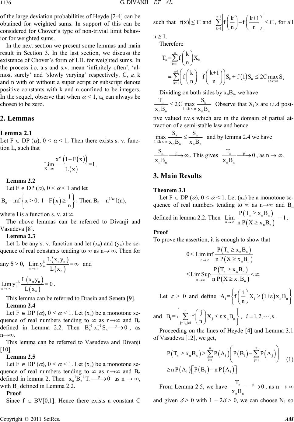 G. DIVANJI ET AL. 1176 of the large deviation probabilities of Heyde [2-4] can be obtained for weighted sums. In support of this can be considered for Chover’s type of non-trivial limit behav- ior for weighted sums. In the next section we present some lemmas and main result in Section 3. In the last section, we discuss the existence of Chover’s form of LIL for weighted sums. In the process i.o, a.s and s.v. mean ‘infinitely often’, ‘al- most surely’ and ‘slowly varying’ respectively. C, , k and n with or without a super script or subscript denote positive constants with k and n confined to be integers. In the sequel, observe that when < 1, ak can always be chosen to be zero. 2. Lemmas Lemma 2.1 Let F DP ( ), 0 < < 1. Then there exists s. v. func- tion L, such that X x1Fx Lim =1 Lx . Lemma 2.2 Let F DP ( ), 0 < < 1 and let n 1 B= infx > 0: 1Fxn . Then Bn = n1/ l(n), where l is a function s. v. at . The above lemmas can be referred to Divanji and Vasudeva [8]. Lemma 2.3 Let L be any s. v. function and let (xn) and (yn) be se- quence of real constants tending to as n . Then for any > 0, nn δ n n n Lxy Lim y= Lx and nn δ n nn Lxy Limy= 0 Lx . This lemma can be referred to Drasin and Seneta [9]. Lemma 2.4 Let F DP ( ), 0 < < 1. Let (xn) be a monotone se- quence of real numbers tending to ∞ as n→∞ and Bn defined in Lemma 2.2. Then p 11 nnn BxS 0 , as n→∞. This lemma can be referred to Vasudeva and Divanji [10]. Lemma 2.5 Let F DP ( ), 0 < < 1. Let (xn) be a monotone se- quence of real numbers tending to ∞ as n→∞ and Bn defined in lemma 2. Then p 11 nnn xB T0 as n → ∞, with Bn defined in Lemma 2.2. Proof Since f BV[0,1]. Hence there exists a constant C such that f(x)≤ C and n-1 k=1 kk+1 ff nn C , for all n ≥ 1. Therefore n nk k=1 n-1 kn 1k n k=1 k T= fX n kk+1 ffS+ f1S2Cmax nn k S Dividing on both sides by xnBn, we have n 1k n nn nn T 2C max xB xB k S Observe that Xi’s are i.i.d posi- tive valued r.v.s which are in the domain of partial at- traction of a semi-stable law and hence k 1k nnn nn SS max xB xB n and by lemma 2.4 we have p n nn S xB . This gives p n nn T0 xB , as n . 3. Main Results Theorem 3.1 Let F DP ( ), 0 < < 1. Let (xn) be a monotone se- quence of real numbers tending to ∞ as n→∞ and Bn defined in lemma 2.2. Then nnn nnn PT xB Lim= 1 n PXxB . Proof To prove the assertion, it is enough to show that nnn nnn nnn nnn PT xB 0< Liminfn PXxB PT xB LimSup< . n PXxB Let > 0 and define iin i A= fX1+εxB n n and n ijnn j=1, ji j B=fX εxB n 1, 2,,in, . Proceeding on the lines of Heyde [4] and Lemma 3.1 of Vasudeva [12], we get, nn nnniij i=1 j=1 11 1 PTxBPA PBPA nP APBnP A (1) From Lemma 2.5, we have p n nn T0 xB , as n and given > 0 with 1 – 2 > 0, we can choose N1 so Copyright © 2011 SciRes. AM 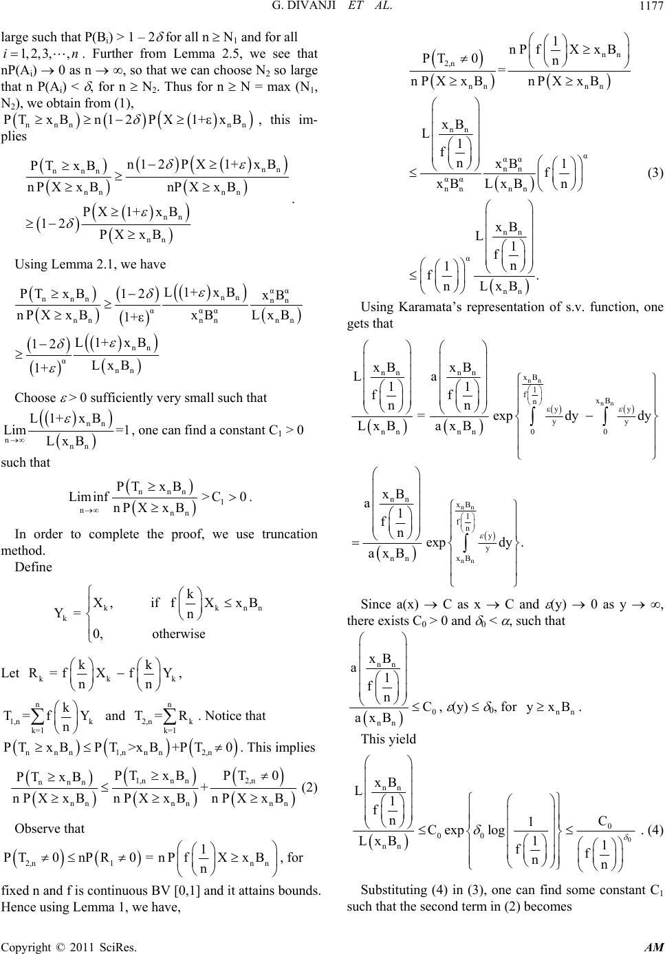 G. DIVANJI ET AL.1177 n large such that P(Bi) > 1 – 2 for all n N1 and for all . Further from Lemma 2.5, we see that nP(Ai) 0 as n , so that we can choose N2 so large that n P(Ai) < , for n N2. Thus for n N = max (N1, N2), we obtain from (1), , this im- plies 1,2, 3,,i nnn PT xB nn n12PX1+εxB nn nnn nn nn nn nn n1 2PX1+xB PT xB nPXx BnPXx B PX1+xB 12 PXxB . Using Lemma 2.1, we have αα nn nnn nn ααα nn nn nn nn α nn L1+ xB PTxB1 2xB nPXx BLx B xB 1+ε L1+ xB 12 LxB 1+ Choose > 0 sufficiently very small such that nn nnn L1+ xB Lim =1 LxB , one can find a constant C1 > 0 such that nnn 1 nnn PT xB Lim inf>C0 nPXx B . In order to complete the proof, we use truncation method. Define kk k k X,if fXxB Y= n 0, otherwise nn Let kk kk R=fXfY nn k , n 1,n k k=1 k T= fY n and . Notice that n 2,n k k=1 T= R nnn1,nnn 2,n PTxBPT >xB+PT0 . This implies 1,nn n2,n nnn nnnn nn PT xBPT0 PT xB+ n PXxBn PXxBn PXxB (2) Observe that 2,n1n n 1 PT0nPR0 =nPfXxB n , for fixed n and f is continuous BV [0,1] and it attains bounds. Hence using Lemma 1, we have, nn 2,n nn nn nn α αα nn αα nn nn nn α nn 1 n PfXxB PT 0n = n PXxBnPXxB xB L1 fnxB 1 f LxBn xB xB L1 fn 1 f. nLxB (3) Using Karamata’s representation of s.v. function, one gets that nn nn nn nn nnnn xB 1 fxB n εyy yy nnnn 00 nn xB 1 fn y y nn xB xB xB La 11 ff nn =expdy dy LxBaxB xB a1 fnexpdy . axB Since a(x) C as x C and (y) 0 as y , there exists C0 > 0 and 0 < , such that nn 0 nn xB a1 fnC axB , (y) 0, for . nn yxB This yield 0 nn 0 00 nn xB L1 fnC 1 Cexp log1 LxB1 ff nn . (4) Substituting (4) in (3), one can find some constant C1 such that the second term in (2) becomes Copyright © 2011 SciRes. AM 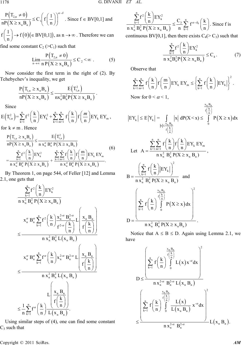 G. DIVANJI ET AL. 1178 - 2,n 1 nn PT 01 Cf nPXx Bn . Since f BV[0,1] and 1 ff0BV[0,1], as n n . Therefore we can find some constant C2 (>C1) such that 2,n 2 nnn PT 0 LimC < nPXx B . (5) Now consider the first term in the right of (2). By Tchebychev’s inequality, we get 2 1,n 1,nn n 22 nn nn nn ET PT xB nPXx Bnx BPXx B . Since nnn 22 2 1,nkk m k=1k=1 m=1 kk ET =fEY+ffEYEY, nnn m for km. Hence 2 1,n 1,nn n nn nn nn nnn 22 kk k=1k=1 m=1 n nnnnnnn ET PT xB nPXx Bn xBPXxB kkm fEY ffEYEY nnn =+ m n xBPXxBn xBPXxB . (6) By Theorem 1, on page 544, of Feller [12] and Lemma 2.1, one gets that n22 k k=1 22 nn nn 2- 2- n2nn nn nn 2- k=1 22 nnnn n2- 2-nn nnnn k=1 22 nnnn k fEY n n xBPXxB xB xB k xBfL kk nff nn n xBLxB xB k xBfxBLk nfn n xBLxB 1k f nn nn n k=1 nn xB Lk fn. Lx B Using similar steps of (4), one can find some constant C3 such that 0 n22 kn- k=1 3 22 k=1 nn nn k fEY Ck nf nn n xBPXxB . Since f is continuous BV[0,1], then there exists C4(> C3) such that n22 k k=1 4 22 nn nn k fEY nC n xBPXxB . (7) Observe that 2 nn n km k k=1 m=1k=1 km k ffEY EYfEY nn n . Now for 0 < < 1, nn nn xB k fn kk xB 0 xk fn EYEY=xdP(X < x)PXxdx Let nn km k=1 m=1 22 nn nn kk ffEY EY nn Anx BP(XxB ) , 2 n k k=1 22 nn nn k fEY n Bnx BP(XxB) and nn 2 xB k fn n k=1 0 22 nn nn k fPXxd n Dnx BP(Xx B) x . Notice that A B D. Again using Lemma 2.1, we have nn nn 2 xB k fn n- k=1 0 2- 2- nn nn 2 xB k fn n- k=1 nn 0 nn 2- 2- nn k fLxxdx n Dnx BLxB Lx k fxdx nLxB Lx B. nx B Copyright © 2011 SciRes. AM 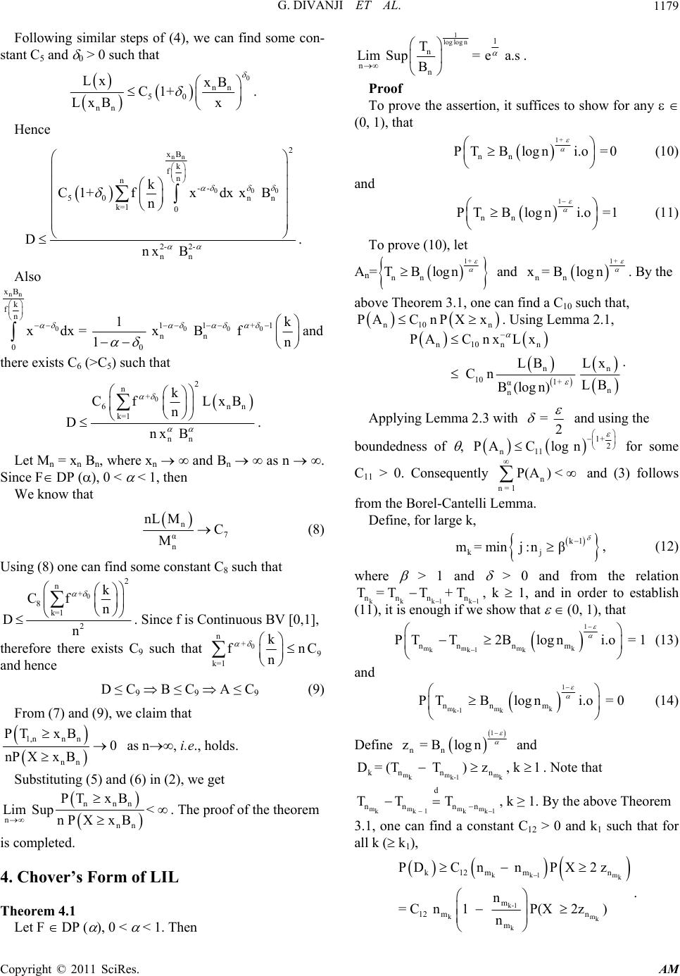 G. DIVANJI ET AL.1179 Following similar steps of (4), we can find some con- stant C5 and 0 > 0 such that 0 nn 50 nn Lx xB C1+ LxB x . Hence nn 000 2 xB k fn n-- 50 nn k=1 0 2- 2- nn k C1+fxdxx B n Dnx B . Also nn 000 xB k fn 11 +1 nn 00 1k xdx = x B f 1n 0 and there exists C6 (>C5) such that 0 2 n+ 6n k=1 nn k Cf LxB n Dnx B n . Let Mn = xn Bn, where xn and Bn as n . Since F DP (), 0 < < 1, then We know that n 7 α n nL MC M (8) Using (8) one can find some constant C8 such that 0 2 n+ 8 k=1 2 k Cf n Dn . Since f is Continuous BV [0,1], therefore there exists C9 such that 0 n+ 9 k=1 k fn n C and hence D ≤ C9 B ≤ C9 A ≤ C9 (9) From (7) and (9), we claim that 1,nn n nn PT xB0 nPXx B as n, i.e., holds. Substituting (5) and (6) in (2), we get nnn nnn PT xB LimSup< n PXxB . The proof of the theorem is completed. 4. Chover’s Form of LIL Theorem 4.1 Let F DP ( ), 0 < < 1. Then 1 log log n1 n nn T LimSup= ea.s B . Proof To prove the assertion, it suffices to show for any (0, 1), that 1+ nn PTBlogni.o =0 (10) and 1 nn PTBlogni.o=1 (11) To prove (10), let An= 1+ nn TBlogn and 1+ nn x= Blogn . By the above Theorem 3.1, one can find a C10 such that, n10n PACnPXx. Using Lemma 2.1, n10nn nn 10 1+ α n n PACnx Lx LB Lx CnLB B(logn) . Applying Lemma 2.3 with = 2 and using the boundedness of , 1+ 2 n11 PAClogn for some C11 > 0. Consequently and (3) follows n n = 1 P(A) < from the Borel-Cantelli Lemma. Define, for large k, k1 kj m= minj:nβ , (12) where > 1 and > 0 and from the relation kkk1 k1 nnn n T= TT+ T , k 1, and in order to establish (11), it is enough if we show that (0, 1), that 1 mm m k kk1k nnnm PTT2Blogni.o = 1 (13) and 1 mm k k-1 k nn m PTBlogni.o = 0 (14) Define 1 nn z = Blogn and mmm kk-1 k kn nn D= (T T)z, k1 1 . Note that mm mm kk 1kk d nn nn TT T , k ≥ 1. By the above Theorem 3.1, one can find a constant C12 > 0 and k1 such that for all k ( k1), kk1 m k k-1 km k k k12mm n m 12 mn m PDCn nPX2 z n = C n1 P(X 2z) n . Copyright © 2011 SciRes. AM 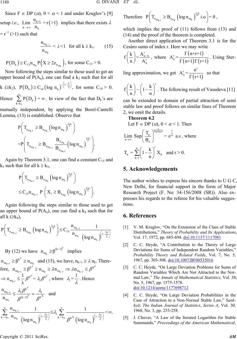 G. DIVANJI ET AL. 1180 Since F DP ( ), 0 < < 1 and under Kruglov’s [9] setup i.e., k+1 k k n Lim=r>1 n implies that there exists = r–1 (>1) such that k1 k m m n<<1 n for all k k1. (15) kk k13m n PDCn PX2z m , for some C13 > 0. Now following the steps similar to those used to get an upper bound of P(An), one can find a k2 such that for all k (k2), 12 k14 k PDC logn , for some C14 > 0. Hence . In view of the fact that Dk’s are 5 k k=k PD = mutually independent, by applying the Borel-Cantelli Lemma, (13) is established. Observe that 1 mm k k-1 k 1 mk mm k k1 k1 mk-1 nn m n nn m n PTBlogn B =PTBlog n. B Again by Theorem 3.1, one can find a constant C15 and k3 such that for all k k3, 1 mm k k-1 k 1 k1m k k nn m 15 m1nm PTBlogn Cn P XBlogn. Again following the steps similar to those used to get an upper bound of P(An), one can find a k4 such that for all k (k4), 1 k1 mm k k1 k k k m nn m153 1 m2 m n1 PTBlognC nlog n By (12) we have implies δ k k1 m nβ k+1 k k m nβn m k and (15), we have, nk+1 nk. There- fore, k+1kk 1k 1 k mmmm nβnn n k-1 kk 1 m1 n= λ , where 1 1 = . Hence k1 1 k k m11 k k1 m n n and k1 1 55 k k m 1 3 1 k = kk = k mk 2 mm n11 <. nlogn logn k 3 1 2 Therefore 1 mmk k-1 k nn m PTBlogni.o= 0 , which implies the proof of (11) follows from (13) and (14) and the proof of the theorem is completed. Another direct application of Theorem 3.1 is for the Cesàro sums of index r. Here we may write r nk r n A k f= nA , where r n Γn+r+1 A= Γn+1 Γr+1. Using Ster- ling approximation, we get r r n n A= Γr+1 so that r k f1 nn k . The following result of Vasudeva [11] can be extended to domain of partial attraction of semi stable law and proof follows on similar lines of Theorem 2, we omit the details. Theorem 4.2 Let F DP ( ), 0 < < 1. Then 1 log log n1 n nn T LimSup= ea.s B , where r n nk k=1 k T = 1X n and r > 0. 5. Acknowledgements The author wishes to express his sincere thanks to U G C, New Delhi, for financial support in the form of Major Research Project (F. No: 34-156/2008 (SR)). Also ex- presses his regards to the referee for his valuable sugges- tions. 6. References [1] V. M. Kruglov, “On the Extension of the Class of Stable Distributions,” Theory of Probability and Its Applications, Vol. 17, 1972, pp. 685-694. doi:10.1137/1117081 [2] C. C. Heyde, “A Contribution to the Theory of Large Deviations for Sums of Independent Random Variables,” Probability Theory and Related Fields, Vol. 7, No. 5, 1967, pp. 303-308. doi:10.1007/BF00535016 [3] C. C. Heyde, “On Large Deviation Problems for Sums of Random Variables Which Are Not Attracted to the Nor- mal Law,” The Annals of Mathematical Statistics, Vol. 38, No. 5, 1967, pp. 1575-1578. doi:10.1214/aoms/1177698712 [4] C. C. Heyde, “On Large Deviation Probabilities in the Case of Attraction to a Non-Normal Stable Law,” Sank- hyā: The Indian Journal of Statistics, Series A, Vol. 30, 1968, No. 3, pp. 253-258. [5] J. Chover, “A Law of the Iterated Logarithm for Stable Summands,” Proceedings of the American Mathematical, Copyright © 2011 SciRes. AM 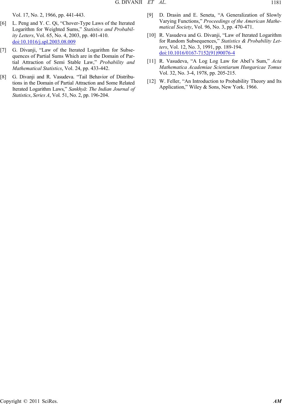 G. DIVANJI ET AL. Copyright © 2011 SciRes. AM 1181 Vol. 17, No. 2, 1966, pp. 441-443. [6] L. Peng and Y. C. Qi, “Chover-Type Laws of the Iterated Logarithm for Weighted Sums,” Statistics and Probabil- ity Letters, Vol. 65, No. 4, 2003, pp. 401-410. doi:10.1016/j.spl.2003.08.009 [7] G. Divanji, “Law of the Iterated Logarithm for Subse- quences of Partial Sums Which are in the Domain of Par- tial Attraction of Semi Stable Law,” Probability and Mathematical Statistics, Vol. 24, pp. 433-442. [8] G. Divanji and R. Vasudeva. “Tail Behavior of Distribu- tions in the Domain of Partial Attraction and Some Related Iterated Logarithm Laws,” Sankhyā: The Indian Journal of Statistics, Series A, Vol. 51, No. 2, pp. 196-204. [9] D. Drasin and E. Seneta, “A Generalization of Slowly Varying Functions,” Proceedings of the American Mathe- matical Society, Vol. 96, No. 3, pp. 470-471. [10] R. Vasudeva and G. Divanji, “Law of Iterated Logarithm for Random Subsequences,” Statistics & Probability Let- ters, Vol. 12, No. 3, 1991, pp. 189-194. doi:10.1016/0167-7152(91)90076-4 [11] R. Vasudeva, “A Log Log Law for Abel’s Sum,” Acta Mathematica Academiae Scientiarum Hungaricae Tomus Vol. 32, No. 3-4, 1978, pp. 205-215. [12] W. Feller, “An Introduction to Probability Theory and Its Application,” Wiley & Sons, New York. 1966.
|