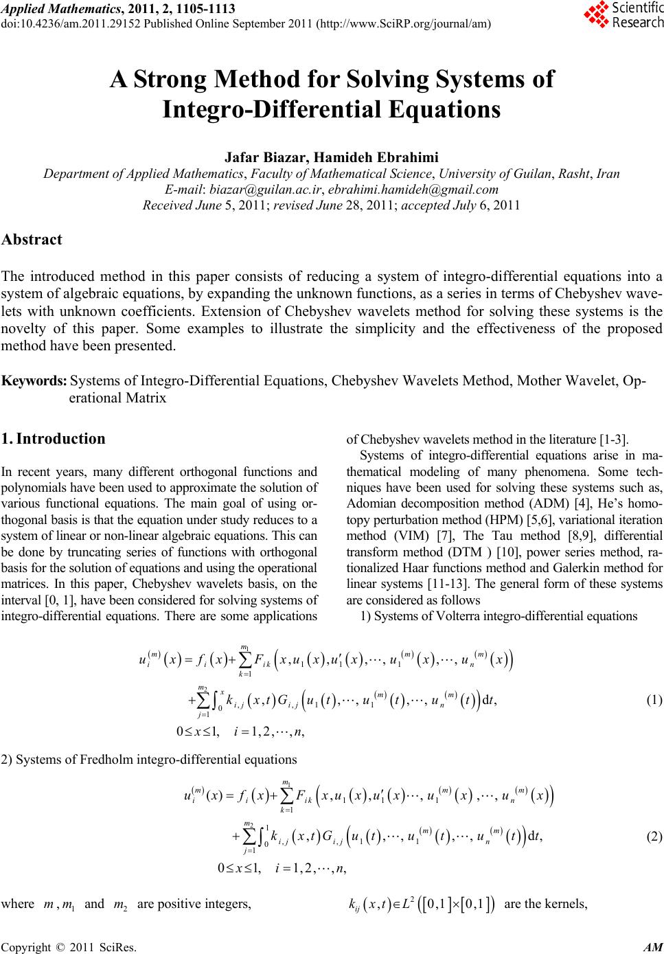
Applied Mathematics, 2011, 2, 1105-1113
doi:10.4236/am.2011.29152 Published Online September 2011 (http://www.SciRP.org/journal/am)
A Strong Method for Solving Systems of
Integro-Differential Equations
Jafar Biazar, Hamideh Ebrahimi
Department of Ap pl i e d M athematics, Faculty of Mathematical Science, University of Guilan, Rasht, Iran
Received June 5, 2011; revised June 28, 2011; accepted July 6, 2011
Abstract
The introduced method in this paper consists of reducing a system of integro-differential equations into a
system of algebraic equations, by expanding the unknown functions, as a series in terms of Chebyshev wave-
lets with unknown coefficients. Extension of Chebyshev wavelets method for solving these systems is the
novelty of this paper. Some examples to illustrate the simplicity and the effectiveness of the proposed
method have been presented.
Keywords: Systems of Integro-Differential Equations, Chebyshev Wavelets Method, Mother Wavelet, Op-
erational Matrix
1. Introduction
In recent years, many different orthogonal functions and
polynomials have been used to approximate the solution of
various functional equations. The main goal of using or-
thogonal basis is that the equation under study reduces to a
system of linear or non-linear algebraic equations. This can
be done by truncating series of functions with orthogonal
basis for the solution of equations and using the operational
matrices. In this paper, Chebyshev wavelets basis, on the
interval [0, 1], have been considered for solving systems of
integro-differential equations. There are some applications
of Chebyshev wavelets method in the literature [1-3].
Systems of integro-differential equations arise in ma-
thematical modeling of many phenomena. Some tech-
niques have been used for solving these systems such as,
Adomian decomposition method (ADM) [4], He’s homo-
topy perturbation method (HPM) [5,6], variational iteration
method (VIM) [7], The Tau method [8,9], differential
transform method (DTM ) [10], power series method, ra-
tionalized Haar functions method and Galerkin method for
linear systems [11-13]. The general form of these systems
are considered as follows
1) Systems of Volterra integro-differential equations

 





 





1
2
11 1
1
,,11
0
1
,,,, ,,
,,,,,
01, 1,2,,,


 

 





m
mm
ii ikn
k
mxmm
ij ijn
j
uxfx Fxuxux ux ux
kxtGut ut utt
xi n

d,
m
d,
m
(1)
2) Systems of Fredholm integro-differential equations

 





 





1
2
11 1
1
1
,,11
0
1
(),,,, ,
,,,,,
01,1,2,,,





 





m
mm
ii ikn
k
mmm
ij ijn
j
uxfxF xuxuxuxux
kxtGut ut utt
xi n
(2)
where , and are positive integers, m1 m2 m








2
,0,10,
ij
kxt L1 are the kernels,

J. BIAZAR ET AL. 1106
,

,1,2,,
i
f
xi n are known functions, ik
F
and
are linear or non-linear functions and
are unknown functions.
ij
G

,1,2,,
i
uxi n,
This paper is organized as follows: in Section 2, Che-
byshev wavelets method is explained. In Section 3, the
application of the method for introduced systems (1) and
(2) is studied. Some numerical examples are presented in
Section 4, Conclusions are presented in Section 5.
2. Wavelets and Chebyshev Wavelets
Wavelets constitute a family of functions constructed
from dilation and translation of a single function called
the mother wavelet [14,15]. When the dilation parameter
a and the translation parameter b vary continuously we
have the following family of continuous wavelets

1
2
,,,,
ab xb
xaab a
a





 0.
(3)
Chebyshev wavelets


,,, , nm

x
knmx  
1
,,2  kk have
four arguments, , is an arbitrary
positive integer andm is the order of Chebyshev
polynomials of the first kind. They are defined on the
interval [0,1], as fo
1,2n
llows:




2
11
,, ,
1
2(2 21),
22
0, otherwise
nm
kk
mkk
xknmx
nn
Txn x




  



,
(4)
where


1,0
π
2,0
π

m
m
m
Tx
Tx m







,
.
1,
(5)
For and .
m are the famous Chebyshev
polynomials of the first kind of degree m, which construct
an orthogonal system with respect to the weight function
0,1,,1mM

,0,1,,TxmM
1
1,2,,2  k n


2
1
1
Wx
x
, on the interval


1,1, and satisfy the
following recursive formula:


 
0
1
11
1,
,
2,
mmm
Tx
Tx x
Tx xTxTxm

 


 
1,2,
.
(6)
The set of Chebyshev wavelets is an orthogonal set with
respect to the weight function


221
k
n
Wx Wxn
A function

f
x defined on the interval [0, 1] may
be presented as
 
10
,
nm nm
nm
f
xc 


 x (7)
where







,n
nmnm Wx
cfx x  . Series presentation
(7), can be approximated by the following truncated se-
ries.
 
1
21
10
,
kMT
nm nm
nm
f
xcxC 



 x
(8)
where C and


x
 are1
2
k1
M
 matrices given by
11
1
10 111 1 202121
T
202 1
T
121 2
,,,, ,,,,
,,,
,,,,,,
C



kk
k
MM
M
MM M
ccc ccc
cc
ccc cc









,





(9)
and


 
 
 
11
1
10111, 12021
T
2, 120 2,1
T
121 2
,,,, ,,
,,,,,
,,,,,,



 









.








kk
k
M
MM
MM M
x
xx xxx
xx x
xxx xx
(10)
Also a function


,
f
xy defined on




0,1 0,1
can be approximated as the following


,.T

f
xyxK y  (11)
Here the entries of matrix 11
22
kk ij
M
M
Kk 


 will
be obtained by
  




,
1
,,,
,1,,2 .
nn
ijij Wy Wx
k
kxfxyy
ij M




,
(12)
The integration of the vector

x
 , defined in (10),
can be achieved as
 
0d
xttP x
 
. (13)
where P is the 11
22
kk
M
M


operational matrix of
integration [1,2]. This matrix is determined as follows.
,







 













L
FF F
OLF
POOL F
F
OOOL
(14)

J. BIAZAR ET AL. 1107
where F, and O
L
are
M
M

matrices given by
 
 
11
2
20
00
22 00
3
2
11 11
200
21 1
11 11
200
22
F







krr
MM
rr
MM













 











 

0
0
,








 







3. Application of Chebyshev Wavelets
Method
In this section the introduced method will be applied to
solve systems (1) and (2).
3.1. Application to Solve System (1)
Consider system of integro-differential Equations (1),
with the following conditions


(15)
00 0
00 0
,
00 0
O










(16)
The property of the product of two Chebyshev wave-
lets vector functions will be as follows



.


T

x
xY Yx   (18)
where is a given vector and is a Y Y11 22
kk
M
M


matrix. This matrix is called the operational matrix of
product. The integration of the product of two Cheby-
shev wavelets vector functions with respect to the weight
function is derived as

,
n
Wx
1
 
0dI
T
n
Wx xxx  
,
1.
(19)


0, 1,,,0,,
s
iis
uainsm


n
.
(20)
First we assume the unknown functions
are approximated in the follow-
ing forms


,1,2,,
m
i
uxi

 
,1,2,,
mT
ii
uxC xin   (21)
Therefore we have

 
1
0
,
!
1, ,,0, ,1.


j
ms
sTms
ii is
j
x
uxCP xa
j
insm






 (22)
Using (20) and (21) other terms will be considered as
the following general expansions




 

 






 




  
11 1
11
12
,
,,,,,, ,,
,
,,,, ,,,
,,
1,2, ,,1,2, ,,1,2, ,.



 

 
T
ii
mm
ikn n
T
ik
mm
T
ijn n ij
T
ij ij
fx Fx
F
xuxux uxuxux
Xx
GututututYt
kxtxKt
ink mjm





 
where is an identity matrix. I
 
 
 

11
2
1
1000
2
21
000 0
44
211
00 0
326
2,
11
21
00 0
21 12121
11
21
000 0
22 22
L







k
rr
MM
rrr r
MM M

















 
 


 










 



0
1


(17)

J. BIAZAR ET AL. 1108
where i
F
and ij
K
are known matrices, ij
X
and
are column vectors of elements of the vectors
.
ij
Y
,1,,
i
Ci n
Substituting these approximations into system (1),
leads to
 
 
 
 

 
1
2
1
2
12
1
0
1
1
0
1
11
12
() d
d
,
1,2, ,,1,2, ,,1,2, ,.
T
 
m
TT T
ii ik
k
mxTT
ij ij
j
m
TT
iik
k
mx
TT
ij ij
j
mm
TT T
iik ijij
kj
CxFxX x
xKtYt t
FxX x
xKtYt t
F
xXx xKPx
inkmjm
 













 
 





11kk
(23)
where are Tij 22
M
M
 
T
Wxx 

matrices.
Multiplying , in to both sides of the
n
1
system (23) and applying

0.d,
x
 a linear or a non-
linear system, in terms of the entries of ,
will be obtained and the elements of vectors
can be obtained by solving this sys-
tem.
,1,2,,
i
Ci n
,1,2,,
i
Ci n
3.2. Solving the System (2)
Consider the system of integro-differential Equations (2)
subject to the conditions (20). To solve this system, let’s
considered the unknown functions
as a linear combination of Chebyshev wavelets, by the
following


,1,2,,
m
i
uxin
.


,1,2,,
mT
ii
ux xCin   (24)
and we have

 

1
0
,
!
1, ,,0,,1


j
ms
ms
sTT
ii
j
x
uxxP Ca
j
ins m






is
(25)
Therefore the following general expansions are
achieved.
 
 

 






 




  
11 1
11
12
,
,,,,, ,,,
,
,,,, ,,,
,,
1,2, ,,1,2, ,,1,2,,.





 
T
ii
mm
ikn n
Tik
mm
T
ijn nij
T
ij ij
fx xF
F
xuxuxuxuxux
xX
Gutu tutu txY
kxtxK t
inkmj m





 
Substitution of these approximations into the system
(2), would be obtained results in
 
 
 
 

 
1
2
1
2
12
1
1
0
1
1
1
0
1
11
() d
d
,
1, 2,...,,
 



 









 






m
TTT
ii ik
k
mTT
ij ij
j
m
TT
iik
k
m
TT
ij ij
j
mm
TTT
iik
kj
xC xFxX
xKttY t
xFx X
xKt ttY
ijij
x
FxXxK
in
DY
(26)
where is a D11 22
kk
M
M


matrix.
Multiplying both sides of the system (26) by




n
Wx x  and applying 0

1.d,
x
 the following
linear or non-linear system will be obtained
12
11
,1, 2,...,,
mm
ii ikijij
kj
CF XKDYin

 
 (27)
Solving system (27) the entries of ,
will be obtained.
,1,2,,
i
Ci n
Also one can check the accuracy of the method. Since
the truncated Chebyshev wavelets series are approximate
the solutions of the systems (1) and (2), so the error
function




i
eu x is constructed as follows


 
1
21
10
.
kMi
iinm nm
nm
eu xu xcx 



 (28)
If we set
j
x
x

where


0,1
j
x, the error values
can be obtained.
4. Numerical Results
In this section some systems of integro-differential equa-
tions are considered and solved by the introduced
method. Parameters and k
M
are considered to be 1
and 6 respectively.
Example 1: Consider the following linear system of
Fredholm integro-differential equations
  
 

  
1
0
2
12
0
23d
3
38,
10
322 d
4
21, 01.
5
 
 




 
 






ux vxxtutvtt
xx
vx uxxtutvtt
xx
(29)

J. BIAZAR ET AL.1109

1
Subject to initial conditions
and .The exact
solutions are and
[8].

01,00,01uu v



2
3uxx

02v

vx321x x
Let’s








 
 
 




 




 

 
 
12
1
22
2
1
2
10
2
2
2
20
2
12
2
12
,,
,
2,
1
,
21
,
2,32
34
38 ,21,
10 5







TT
TT
TTTT T
TT
TT T
TT
TT T
TT
TT
ux xCvx xC
ux xPC
vx xPCxPC xV
uxx PC
xP CxU
vxx PCx
xP CxV
1
,
x
txKt xtxKt
xx xFxxF







 

 

 





 
Substituting into (28), the following linear system will
be obtained
 

 

121
22
11020
12
22
210 20
33
2(2 .
T
TT
T
TT
CPCV
KDPC UPCVF
PC C
1
2
,
K
DP CUP CVF












.
Solving this system; the solutions would be achieved
as follows
 

22
113 1,
TT
uxx PCx  
 

23
22121
TT
vxx PCxxx  
This is the exact solution.
Example 2: Consider the following non-linear system
of Fredholm integro-differential equations with the exact
solutions and

21ux x

e
x
vx and boundary
conditions




01, 00
,
uu


and

01v


01v

.
  

 

12
0
13
0
233
42d
213
4e 2e,
15 6
1
3d
2
71 119
e3eee ,
66 918
01,
x
x
uxvxxtutxtvt t
xx
vxuxxtutvtxtvt t
xx x
x
 
 





 
 


 







(30)
In this example, let’s take




 
 
 
 




1
2
1
22
22
11
,
,
,
1,
1





T
T
TT
TTTT T
TTTTT
ux xC
vx xC
ux xPC
vx xPCxPCxV
uxxPCx PCxV








 

1
1

 





 
 
 
 


2
2
2
20
2
12
3
3
12
3
1
233
2
1
,
,,
,
,2 ,
,
213
4e 2e,
15 6
71 119
e3eee
66 918




 









 







TT
TTT
TT
T
TT
T
xT
xT
vxx PCx
xP CxV
uxxY uxvxxY
vx xY
xtxK txtxKt
xtxKt
xx xF
.
x
xx xF
Applying the Chebyshev wavelets method, the fol-
lowing non-linear system will be obtained
 

2
12011221
2
2113213
44
11
33
22
TT
T
CPCVKDYKDPCVF
CPCVKDYKDYF
1
2
,
.

 




Solving this system the following results would be
achieved.
1,0 1,1
7
1,21, 3
77
1, 41, 5
2,0 2,1
2,2 2,3
2.506705578,0.00009696248441,
0.00001788458767,5.080260046 10,
1.44917065510 ,2.37389501710 ,
2.197451850, 0.7536322881,
0.09324678580, 0.0077327666
cc
cc
cc
cc
cc




 


2,4 2,5
17,
0.0004818914245, 0.00002403741177.cc

Therefore, the following approximate solutions will be
achieved.


54
32
8
0.000001345778125 0.00001026370827
0.00001182646441 0.9999858747
1.336715265 101,
ux
x
x
x
xx








54
32
0.01391739110 0.03477166926
0.1704167644 0.49905851211.





xx
xx
v
x
x
Plots of the exact and approximate solutions are pre-

J. BIAZAR ET AL. 1110
sented in Figure 1 and also plots of error functions are
shown in Figure 2.
Example 3: consider non-linear system of Volterra
integro-differential equations with conditions






00,01,00,uuu

.




01, 00vv

 and

01.v 
 

  
22
0
2
0
d,
1
sinsind ,01.
2
x
x
uxxuxut vtt
vxxx utvttx
 
 


 
 



(31)
The exact solutions are and
[7].

sinux x
C

cosvx x
Entries of vectors 1 C and 2 are computed by
solving a system of nonlinear equations with six un-
knowns and six equations as follows
1,0 1,1
1,21, 3
1, 41, 5
2,0 2,1
2,2 2,3
2,
1.032210259.2058700709
0.04760379553 0.002178545560
0.0002500199685 0.000006823287551
.5638994174 .3768424359
0.0260060615
,,
,,
,,
7 0.00398782176
,0,
,,4
0
cc
cc
cc
cc
cc
c









42,5
0.00013658879930.0000141989 5,.04 9c
Therefore, one gets the following approximate solutions
 
3
32
7
1
54
0.007222202515 0.001672032401
0.1676491115 0.0002483913114
0.3210839427 10,
T
x
x
x
x
uxCPx x
x










 
2
3
4
3
2
5
2
0.003945506187 0.04597489600
1
0.002189489246 2
0.000042656686 10
1
2
1.
T
x
x
xx
x
xC
x
vPx  


 


Approximate and exact solutions are plotted in Figure
3. Error functions are plotted in Figure 4.
Example 4: Consider the following non-linear system
of Volterra integro-differential equations with the exact
solutions ,

2
ux x

vx x

and on

2
3wxx
01
x
 [5].
 


 

  
 

322
0
2
0
32 2
223
0
22 d
3d
,
4
22
3
d,
x
x
x
uxxxvxv tutwtt
vxxxutxtvtutwtt
wxxutu x
xvtuttwtt
 
 

 
 



 
 








,
(32)
(a)
(b)
Figure 1. (a) and (b) plots of exact and approximate solu-
tions of Example 2.
Figure 2. Plots of error functions of Examples 2.

J. BIAZAR ET AL.1111
(a)
(b)
Figure 3. (a) and (b) plots of exact and approximate solu-
tions of Example 3.
Figure 4. Plots of error functions of Examples 3.
(a)
(b)
(c)
Figure 5. (a), (b) and (c) plots of exact and approximate
solutions of Example 4.

J. BIAZAR ET AL. 1112
Figure 6. Plots of error functions of Examples 4.
Initial conditions are

00,00uu
,



00

0w
and .
 
00,01vv

,w0
The following approximate solutions would be achie-
ved by using Chebyshev wavelets method.
 
11 5104
11 3
2
2
5
1
3
1
8.527181902102.509321144 10
4.653979568 103.641136902 10
6.5519429650 ,1
T
ux
x
x
P
x
x
Cx
1
x




 






 
11 5104
1
2
2
03 102
14
7.880203686101.637978948 10
1.014393404 103.511874249 10
1.461792049 10,
T
x
x
x
x
vxCPx x
x






 



1 4
 
10 59 4
10 3
2
2
1
3
2
4.043702026101.228923763 10
7.249989732 103.000000001
1.753892960 102.9553106520.1
T
wx CP
x
x
xx
x
x










Plots of the exact solution, approximate solution and
error functions are shown in Figures 5 and 6.
5. Conclusions
This paper proposes a powerful technique for solving
systems of integro-differential equations using Cheby-
shev wavelets method. Comparison of the approximate
solutions and the exact solutions shows that the proposed
method is more efficient tool and more practical for
solving linear and non-linear systems of integro-difieren-
tial equations, and plots confirm. Researches for finding
more applications of this method and other orthogonal
basis functions are one of the goals in our research group.
The package Maple 13 has been used to carry the com-
putations associated with these examples.
6. Acknowledgements
Authors are grateful to the anonymous reviewers for his
(her) influential comments which have improved the
quality of the paper.
7. References
[1] E. Babolian and F. Fattahzadeh, “Numerical Computation
Method in Solving Integral Equations by Using Cheby-
shev Wavelet Operational Matrix of Integration,” Applied
Mathematics and Computations, Vol. 188, No. 1, 2007,
pp. 1016-1022. doi:10.1016/j.amc.2006.10.073
[2] E. Babolian and F. Fattahzadeh, “Numerical Solution of
Differential Equations by Using Chebyshev Wavelet Op-
erational Matrix of Integration,” Applied Mathematics
and Computations, Vol. 188, No. 1, 2007, pp. 417-426.
[3] Y. Li, “Solving a Nonlinear Fractional Differential Equa-
tion Using Chebyshev Wavelets,” Communications in
Nonlinear Science and Numerical Simulation, Vol. 15,
No. 9, 2010, pp. 2284-2292.
doi:10.1016/j.cnsns.2009.09.020
[4] J. Biazar, “Solution of Systems of Integral-Differential
Equations by Adomian Decomposition Method,” Applied
Mathematics and Computation, Vol. 168, No. 2, 2005, pp.
1232-1238. doi:10.1016/j.amc.2004.10.015
[5] J. Biazar, H. Ghazvini and M. Eslami, “He’s Homotopy
Perturbation Method for Systems of Integro-Differential
Equations,” Chaos, Solitions and Fractals, Vol. 39, No. 3,
2009, pp. 1253-1258. doi:10.1016/j.chaos.2007.06.001
[6] E. Yusufoglu (Agadjanov), “An Efficient Algorithm for
Solving Integro-Differential Equations System,” Applied
Mathematics and Computation, Vol. 192, No. 1, 2007, pp.
51-55. doi:10.1016/j.amc.2007.02.134
[7] J. Biazar and H. Aminikhah, “A New Technique for
Solving Integro-Differential Equations,” Computers and
Mathematics with Applications, Vol. 58, No. 11-12, 2009,
pp. 2084-2090. doi:10.1016/j.camwa.2009.03.042
[8] J. Pour-Mahmoud and M. Y. Rahimi-Ardabili and S. Sha-
morad, “Numerical Solution of the System of Fredholm
Integro-Differential Equations by the Tau Method,” Ap-
plied Mathematics and Computation, Vol. 168, 2005, pp.
465-478.
[9] S. Abbasbandy and A. Taati, “Numerical Solution of the
System of Nonlinear Volterra Integro-Differential Equa-
tions with Nonlinear Differential Part by the Operational
Tau Method and Error Estimation,” Journal of Computa-
tional and Applied Mathematics, Vol. 231, No. 1, 2009,
pp. 106-113. doi:10.1016/j.cam.2009.02.014
[10] A. Arikoglu and I. Ozkol, “Solutions of Integral and In-
tegro-Differential Equation Systems by Using Differen-
tial Transform Method,” Computers and Mathematics

J. BIAZAR ET AL. 1113
with Applications, Vol. 56, No. 9, 2008, pp. 2411-2417.
doi:10.1016/j.camwa.2008.05.017
[11] M. Gachpazan, “Numerical Scheme to Solve Integro-
Difierential Equations System,” Journal of Advanced Re-
search in Scientific Computing, Vol. 1, No. 1, 2009, pp.
11-21.
[12] K. Maleknejad, F. Mirzaee and S. Abbasbandy, “Solving
Linear Integro-Differential Equations System by Using
Rationalized Haar Functions Method,” Applied Mathe-
matics and Computation, Vol. 155, No. 2, 2004, pp. 317-
328. doi:10.1016/S0096-3003(03)00778-1
[13] K. Maleknejad and M. Tavassoli Kajani, “Solving Linear
Integro-Differential Equation System by Galerkin Meth-
ods with Hybrid Functions,” Applied Mathematics and
Computation, Vol. 159, No. 3, 2004, pp. 603-612.
doi:10.1016/j.amc.2003.10.046
[14] I. Daubeches, “Ten Lectures on Wavelets,” SIAM,
Philadelphia, 1992.
[15] Ole Christensen and K. L. Christensen, “Approximation
Theory: From Taylor Polynomial to Wavelets,” Birk-
hauser, Boston, 2004.