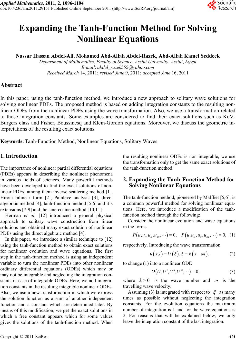
Applied Mathematics, 2011, 2, 1096-1104
doi:10.4236/am.2011.29151 Published Online September 2011 (http://www.SciRP.org/journal/am)
Expanding the Tanh-Function Method for Solving
Nonlinear Equations
Nassar Hassan Abdel-All, Mohamed Abd-Allah Abdel-Razek, Abd-Allah Kamel Seddeek
Department of Mat hematics, Faculty of Science , Assiut University, Assiut, Egypt
Received March 14, 201 1; revised June 9, 2011; accepted June 16, 2011
Abstract
In this paper, using the tanh-function method, we introduce a new approach to solitary wave solutions for
solving nonlinear PDEs. The proposed method is based on adding integration constants to the resulting non-
linear ODEs from the nonlinear PDEs using the wave transformation. Also, we use a transformation related
to those integration constants. Some examples are considered to find their exact solutions such as KdV-
Burgers class and Fisher, Boussinesq and Klein-Gordon equations. Moreover, we discuss the geometric in-
terpretations of the resulting exact solutions.
Keywords: Tanh-Fun cti on M eth od, Nonlinea r Equations, Solitary Waves
1. Introduction
The importance of nonlinear partial differential equ ation s
(PDEs) appears in describing the nonlinear phenomena
in various fields of sciences. Many powerful methods
have been developed to find the exact solutions of non-
linear PDEs, among them inverse scattering method [1],
Hirota bilinear form [2], Painlevé analysis [3], direct
algebraic method [4], tanh-function method [5,6] and it’s
extensions [7-9] and the sine-cosine method [10,11].
Herman et al. [12] introduced a general physical
approach to solitary wave construction from linear
solutions and obtained many exact solution of nonlinear
PDEs using the direct algebraic method [4].
In this paper, we introduce a similar technique to [12]
using the tanh-function method to obtain exact solutions
for nonlinear evolution and wave equations. The first
step in the tanh-function method is using an independent
variable to turn the nonlinear PDEs into other nonlinear
ordinary differential equations (ODEs) which may or
may not be integrable and neglecting the integration con-
stants in case of integrable ODEs. Here, we add integra-
tion constants in the resu lting integr able non linear ODEs.
Also, we use a new transformation in which we express
the solution function as a sum of another independent
function and a constant which are determined later. By
means of this modification, we get the exact solutions in
which a free constant appears which for some values
gives the solutions of the tanh-function method. When
the resulting nonlinear ODEs is non integrable, we use
the transformation only to get the same exact solutions of
the tanh-function method.
2. Expanding the Tanh-Function Method for
Solving Nonlinear Equations
The tanh-function method, pioneered by Malfliet [5,6], is
a common powerful method for solving nonlinear equa-
tions. Here, we introduce a modification of the tanh-
function method through the following:
Consider the nonlinear evolution and wave equations
in the forms

 
,,, ,=0,,,, ,=0,
txxx ttxxx
Puuu uPuu u u (1)
respectively. Introducing the wave transformation




,= ,=,uxt Ukxt


   (2)
to change (1) into a nonlinear ODE


,,, ,=0,OUU UU

 (3)
where is the wave number and >0k

is the
travelling wave velocity.
Assuming (3) is integrated with resp ect to

as many
times as possible without neglecting the integration
constants. For the evolution equations the maximum
number of integration is 1 and for the wave equations is
2. For reasons that will be explained below, we only
leave the integration con s tant of the last integration.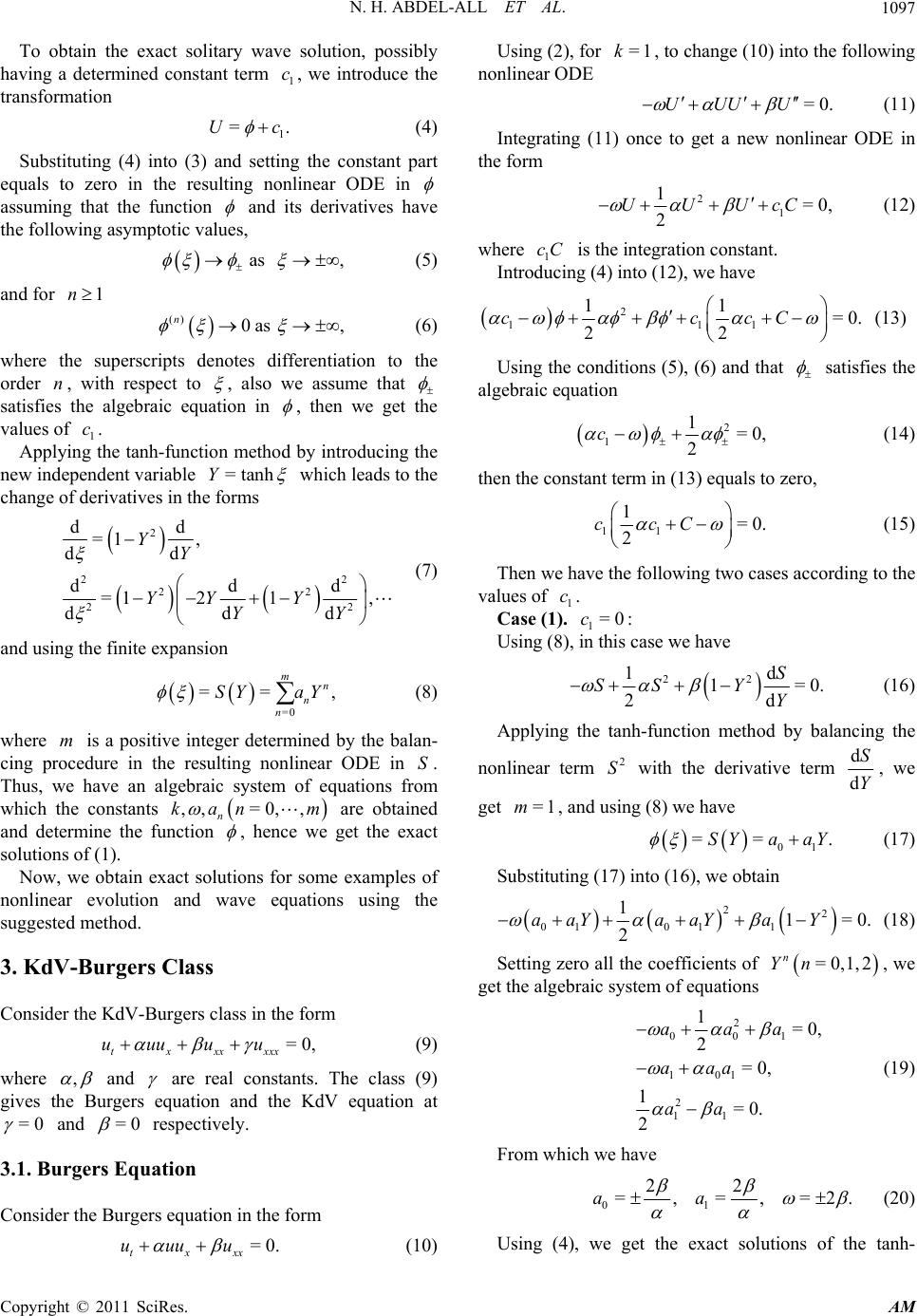

N. H. ABDEL-ALL ET AL.1097
.c
To obtain the exact solitary wave solution, possibly
having a determined constant term , we introduce the
transformation 1
c
1
=U

 (4)
Substituting (4) into (3) and setting the constant part
equals to zero in the resulting nonlinear ODE in

assuming that the function

and its derivatives have
the following asymptotic values,

as ,  



(5)
and for 1n

() 0as , n
   (6)
where the superscripts denotes differentiation to the
order , with respect to n

, also we assume that


satisfies the algebraic equation in

, then we get the
values of .
1
Applying the tanh-function method by introducing the
new independent variable
c
=tanhY

which leads to the
change of derivatives in the forms

 
2
2
22
22
dd
=1 ,
dd
dd
=12 1,
d dd
YY
YY Y
YY




 



2
d



,
(7)
and using the finite ex pansion
 
=0
==
mn
n
n
SY aY 
 (8)
where is a positive integer determined by the balan-
cing procedure in the resulting nonlinear ODE in .
Thus, we have an algebraic system of equations from
which the constants
mS


,,=0, ,
n
kan m   are obtained
and determine the function

, hence we get the exact
solutions of (1).
Now, we obtain exact solutions for some examples of
nonlinear evolution and wave equations using the
suggested method.
3. KdV-Burgers Class
Consider the KdV-Burgers class in the form
=0,
txxx xxx
uuuu u

  (9)
where ,

 and

are real constants. The class (9)
gives the Burgers equation and the KdV equation at
=0

and =0

respectively.
3.1. Burgers Equation
Consider the Burgers equation in the form
=0.
txxx
uuuu

  (10)
Using (2), for , to change (10) into the following
nonlinear ODE =1k
=0.UUUU





 (11)
Integrating (11) once to get a new nonlinear ODE in
the form
21
1=0,
2
UUUcC 
   (12)
where is the integration constant.
1
Introducing (4) into (12), we have
cC

2
111
11
=0.
22
ccc   


 


C (13)
Using the condition s (5), (6) and that

 satisfies the
algebraic equation

2
11=0,
2
c 

 (14)
then the constant term in (13) equals to zero,
11
1=0.
2
ccC







(15)
Then we have the following two cases according to the
values of .
1
Case (1).
c
1
Using (8), in this case we have
=0:c

22
1
1
d
=0
2d
S
SS Y
Y
  . (16)
Applying the tanh-function method by balancing the
nonlinear term with the derivative term
2
Sd
d
S
Y, we
get , and using (8) we have =1m


01
==SYa aY  . (17)
Substituting (17) in to (16), we obtain


22
0101 1
11=0
2
aaYaaYa Y   . (18)
Setting zero all the coefficients of , we
get the algebraic system of equations

=0,1,2
n
Yn
2
001
101
2
11
1=0,
2=0,
1=0.
2
aaa
aaa
aa



 


(19)
From which we have
01
22
=,=,=2.aa




 (20)
Using (4), we get the exact solutions of the tanh-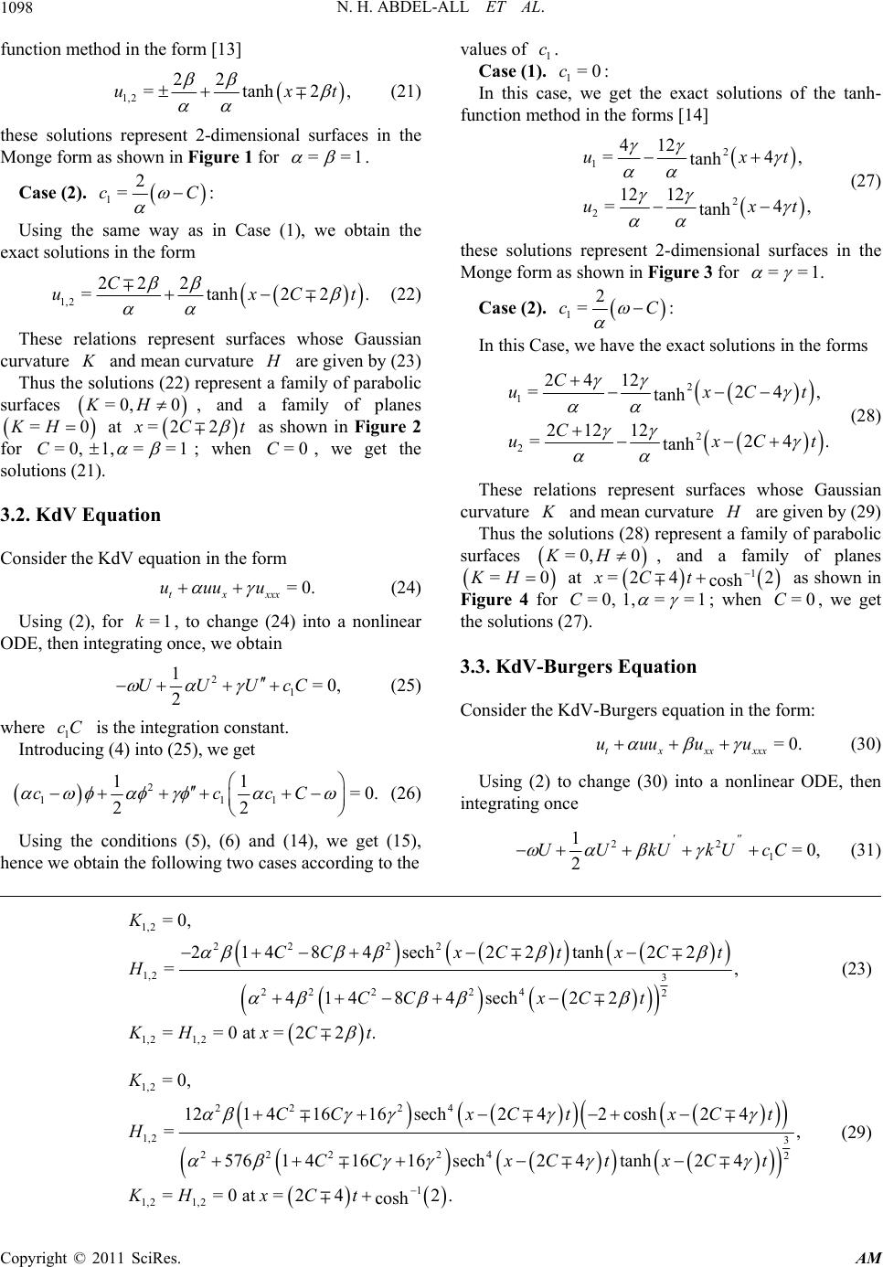

N. H. ABDEL-ALL ET AL. 1098
function method in the form [13] values of .

1,2 22
=tanhux


2,t


  (21)
1
Case (1).
c
1
In this case, we get the exact solutions of the tanh-
function method in the forms [14]
=0:c
these solutions represent 2-dimensional surfaces in the
Monge form as shown in Figure 1 for ==1

 .


2
1
2
2
412
=4
tanh
12 12
=4
tanh
ux
ux
 


,
,
t
t




(27)
Case (2).

12
=:cC



Using the same way as in Case (1), we obtain the
exact solutions in th e form
 
1,2 22 2
=tanh2
C
ux
 




2.Ct (22)
these solutions represent 2-dimensional surfaces in the
Monge form as shown in Figure 3 for ==1.


Case (2).

12
=:cC 


These relations represent surfaces whose Gaussian
curvature and mean curvature
K
H
are given by (23) In this Case, we have the exact solutions in the forms
 
 
2
1
2
2
2412
=2
tanh
21212
=2
tanh
C
ux
C
ux
 

 



Thus the solutions (22) represent a family of parabolic
surfaces , and a family of planes
at

=0, 0KH

0=2
4,
4.
Ct
Ct
(28)


=KH

2
x
Ct

 as shown in Figure 2
for =0C,1,==1

 ; when , we get the
solutions (21). =0C
These relations represent surfaces whose Gaussian
curvature and mean curvature
K
H
are given by (2 9)
3.2. KdV Equation Thus the solutions (28) represent a family of parabolic
surfaces


=0, 0KH

, and a family of planes


0=KH

at


1
4 2
cos h
xCt  
= =1
Consider the KdV equation in the form

=2
=0,1,C as shown in Figure 4 for

 C; when , we get
the solutions (27). =0
=0.
tx xxx
uuuu

  (24)
Using (2), for , to change (24) into a nonlinear
ODE, then int egratin g once, we obtain
=1k
3.3. KdV-Burgers Equation
21
1=0,
2
UUUcC 

  (25)
Consider the KdV-Burgers equation in the form:
where is the integration constant.
1
Introducing (4) into (25), we get
cC =0.
txxx xxx
uuuu u


 (30)

2
111
11
=0.
22
cccC  


 


(26) Using (2) to change (30) into a nonlinear ODE, then
integrating once
22
1
1=0,
2
'''
UUkUkUcC    (31)
Using the conditions (5), (6) and (14), we get (15),
hence we obtain the fo llowing two cases according to the






 


1,2
22 22
1,2 3
2222 42
1,2 1,2
=0,
214 84sech22tanh22
=,
414 84sech22
==0 at =22.
K
CCxCtxC t
H
CCxC t
KHxC t
 
 






(23)







   
 
 
1,2
22 24
1,2 3
222 242
1
1,2 1,2
=0,
12141616sech2 42cosh2 4
= ,
576141616sech2 4tanh2 4
==0 at =242.
cosh
K
CCxC txC t
H
CCxC txC t
KH xCt
 
 


 






(29)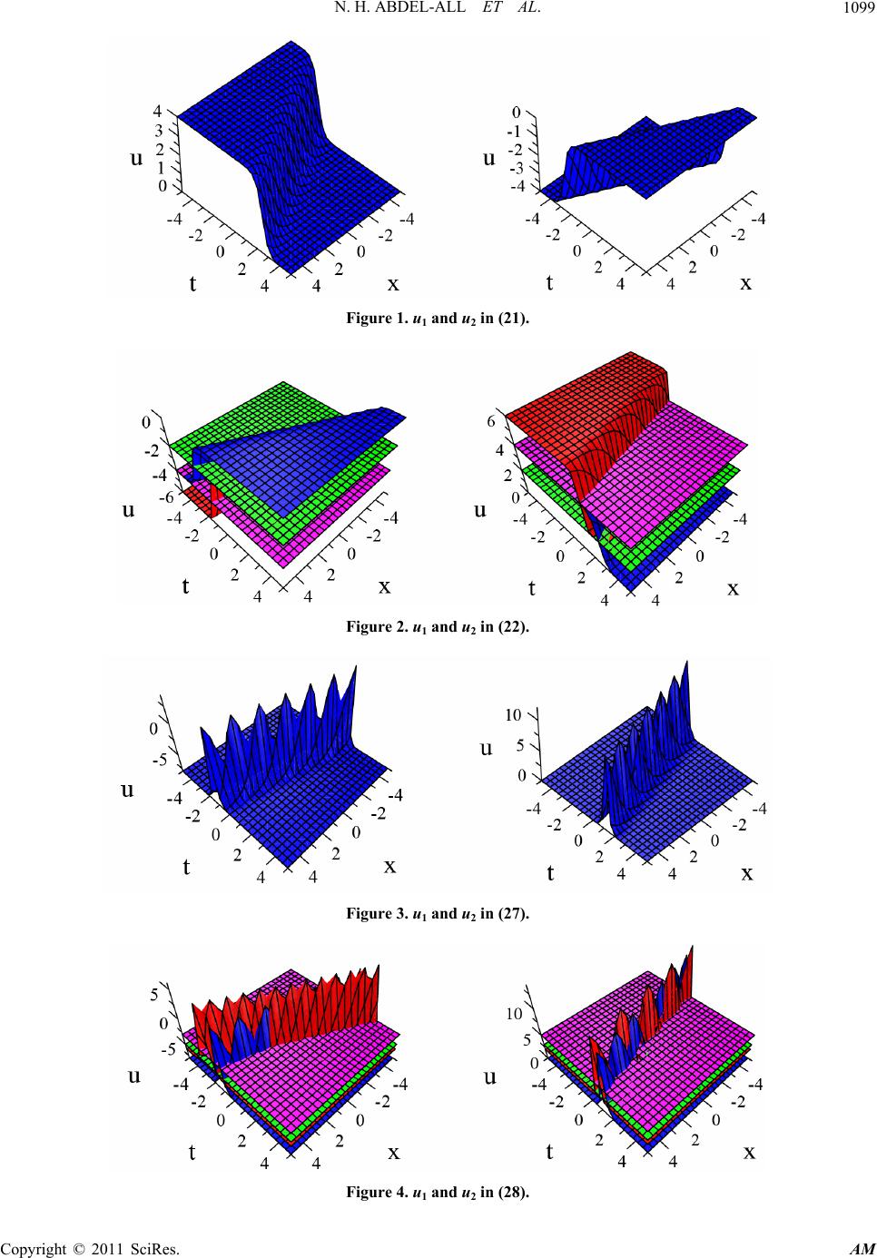

N. H. ABDEL-ALL ET AL.1099
Figure 1. u1 and u2 in (21).
Figure 2. u1 and u2 in (22).
Figure 3. u1 and u2 in (27).
Figure 4. u1 and u2 in (28).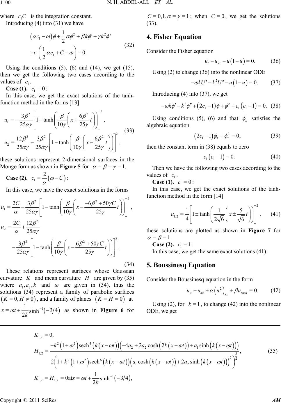

N. H. ABDEL-ALL ET AL. 1100
where is the integration constant.
1
Introducing (4) into (31) we have
cC =0,1, = =1C

 ; when , we get the solutions
3). =0C

22
1
11
1
2
1=0.
2
ck
ccC
k







 




(3
4. Fisher Equation

(32)
Consider the Fisher equation

1=
txx
uu uu 0
0.
. (36)
Using the conditions (5), (6) and (14), we get (15),
then we get the following two cases according to the
values of .
Using (2) to change (36) into the nonlinear ODE

21=kUkUuu

  (37)
1
Case (1).
c
1
In this case, we get the exact solutions of the tanh-
function method in the forms [13]
=0:cIntroducing (4) into (37), we get
2
22
1
2
22 2
2
36
=1tanh ,
2510 25
12 36
=1tanh
25 251025
uxt
ux

 

 



  










 










22
111
21 1=0kk ccc  
 .
(38)
,t









.
(33)
Using conditions (5), (6) and that

 satisfies the
algebraic equation


2
1
21 =0c 

 , (39)
then the constant term in (38) equals to zero


111=0.cc (40)
these solutions represent 2-dimensional surfaces in the
Monge form as shown in Figure 5 for ===1

 Then we have the following two cases according to the
values of .
Case (2).

12
=:cC 

 1
Case (1).
c
In this case, we have the exact solutions in the forms
2
22
1
2
2
2
22
23 650
=1tanh
2510 25
212
=25
3650
1tanh .
2510 25
CC
ux
C
u
C
xt

 



 




 










1
In this case, we get the exact solutions of the tanh-
function method in the form [14]
=0:c
,t



  







2
1,2 115
=1tanh
426 6
ux,t















 (41)

these solutions are plotted as shown in Figure 7 for
==1.


Case (2).
1
In this case, we get the same exact solutions (41).
=1:c
5. Boussinesq Equation
(34)
These relations represent surfaces whose Gaussian
curvature and mean curvature K
H
are given by (35)
Consider the Boussinesq equation in the form
where 12 and ,,aak

are given in (34), thus the
solutions (34) represent a family of parabolic surfaces
, and a family of planes

, 0KH

2=0.
tt xxxxxx
xx
uu uu    (42)

=0

=0KH

at Using (2), for , to change (42) into the nonlinear
ODE, we get =1k

1

=3 4
sinh
2
xtk



1 as shown in Figure 6 for









     


1,2
22422 1
1,2 3
22
22612
1
1,2 1,2
=0,
1sech42cosh2 sinh
= ,
2 11sechcosh2sinh
1
==0at= 34,
sinh
2
K
kkx taakxtakx t
H
kkxtakxt akxt
KH xt
k
 
 


 






(35)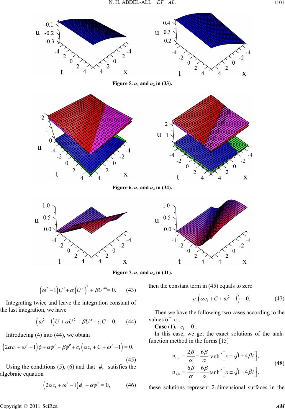

N. H. ABDEL-ALL ET AL.1101
Figure 5. u1 and u2 in (33).
Figure 6. u1 and u2 in (34).
Figure 7. u1 and u2 in (41).
 
22
1=UU U 

 
0.
=0.

=0.
(43)
Integrating twice and leave the integration constant of
the last integration, we have

22
1
1UU UcC 

 (44)
Introducing (4) into (44), we obtain
 
22 2
111
21 1cccC  

 
(45)
Using the condition s (5), (6) and that

 satisfies the
algebraic equation

22
1
21c  

 
then the constant term in (45) equals to zero


2
11 1=0.ccC
   (47)
Then we have the following two cases according to the
values of .
1
Case (1). :
c
1
In this case, we get the exact solutions of the tanh-
function method in the forms [15]
=0c
2
1,2
2
3,4
26
=1
tanh
66
=1
tanh
ux
ux

4,
4,
t
t











(48)
=0, (46) these solutions represent 2-dimensional surfaces in the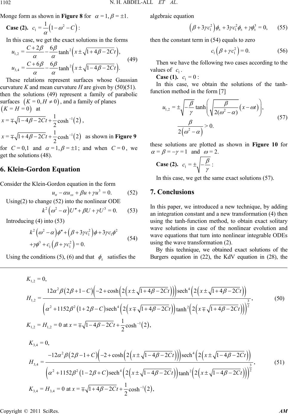

N. H. ABDEL-ALL ET AL. 1102
Monge form as shown in Figure 8 for =1,= 1.



Case (2).

2
11
=1cC


:
In this case, we get the exact solutions in the forms


2
1,2
2
3,4
26
=1
tanh
66
=1
tanh
C
ux
C
ux
 

 




42,
42.
Ct
Ct

(49)
These relations represent surfaces whose Gaussian
curvature K and mean curvature H are given by (50)(51).
then the solutions (49) represent a family of parabolic
surfaces , and a family of planes
at

=0,0KH

==0KH

1
1
=142 2
cosh
2
xCt 

 ,

1
1
=142 2
cosh
2
xCt


  as shown in Fi g u re 9
for and = 0,1C=1,= 1



; and when , we
get the solutions (48). =0C
6. Klein-Gordon Equation
Consider the Klein-Gordon equation in the form
3=0.
tt xx
uu uu   (52)
Using(2) to change (52) into the nonlinear ODE

22 3
=0.kUUU  

 (53)
Introducing (4) into (53)





22 2
1
32
11
33
=0.
kc
cc
2
1
c

 
 

 
  (54)
Using the conditions (5), (6) and that

 satisfies the
algebraic equation


223
11
33cc  

=0, (55)
then the constant term in (54) equals to zero


2
11
=0.cc   (56)
Then we have the following two cases according to the
values of .
1
Case (1). :
c
1
In this case, we obtain the solutions of the tanh-
function method in the form [7]
=0c


1,2 2
2
=tanh
2( )
>0.
2
ux






 





, t
(57)
these solutions are plotted as shown in Figure 10 for
== =1



and =2.

Case (2). 1=:c



In this case, we get the same exact solutions (57).
7. Conclusions
In this paper, we introduced a new technique, by adding
an integration constant and a new transformation (4) then
using the tanh-function method, to obtain exact solitary
wave solutions in case of the nonlinear evolution and
wave equations that turn into nonlinear integrable ODEs
using the wave transformation (2).
By this technique, we obtained exact solutions of the
Burgers equation in (22), the KdV equation in (28), the













1,2
2 4
1,2 3
2
22 42
1
1,2 1,2
=0,
12212cosh21 42sech2142
= ,
115212sech21422142
tanh
1
==0 at =1422,
cosh
2
K
CxCtx
H
CxCt xCt
KH xCt
 
 


  
 
 


Ct
(50)


 






 

3, 4
2 4
3,4 3
2
22 42
1
3,4 3,4
=0,
12212cosh21 42sech2142
= ,
11521 2sech21 4221 42
tanh
1
==0 at =1422,
cosh
2
K
CxCtx
H
Cx Ctx Ct
KH xCt
 
 


 

 
Ct
(51)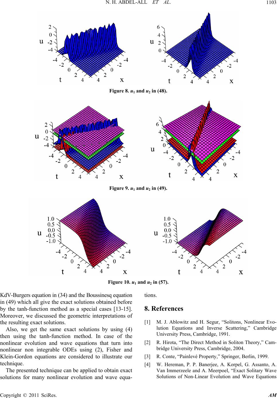

N. H. ABDEL-ALL ET AL.1103
Figure 8. u1 and u2 in (48).
Figure 9. u1 and u2 in (49).
Figure 10. u1 and u2 in (57).
KdV-Burgers equation in (34) and the Boussinesq equation
in (49) which all give the exact solutions obtained before
by the tanh-function method as a special cases [13-15].
Moreover, we discussed the geometric interpretations of
the resulting exact solutions.
Also, we get the same exact solutions by using (4)
then using the tanh-function method. In case of the
nonlinear evolution and wave equations that turn into
nonlinear non integrable ODEs using (2), Fisher and
Klein-Gordon equations are considered to illustrate our
technique.
The presented technique can be applied to obtain exact
solutions for many nonlinear evolution and wave equa-
tions.
8. References
[1] M. J. Ablowitz and H. Segur, “Solitons, Nonlinear Evo-
lution Equations and Inverse Scattering,” Cambridge
University Press, Cambridge, 1991.
[2] R. Hirota, “The Direct Method in Soliton Theory,” Cam-
bridge University Press, Cambridge, 2004.
[3] R. Conte, “Painlevé Property,” Springer, Berlin, 1999.
[4] W. Hereman, P. P. Banerjee, A. Korpel, G. Assanto, A.
Van Immerzeele and A. Meerpoel, “Exact Solitary Wave
Solutions of Non-Linear Evolution and Wave Equations

N. H. ABDEL-ALL ET AL. 1104
Using a Direct Algebraic Method,” Journal of Physics A:
Mathematical and General, Vol. 19, No. 5, 1986, pp.
607-628. doi:10.1088/0305-4470/19/5/016
[5] W. Malfliet, “Solitary Wave Solutions of Nonlinear
Wave Equations,” American Journal of Physics, Vol. 60,
No. 7, 1992, pp. 650-654. doi:10.1119/1.17120
[6] W. Malfliet and W. Hereman, “The Tanh Method: I Ex-
act Solutions of Nonlinear Evolution and Wave Equa-
tions,” Physica Scripta, Vol. 54, No. 6, 1996, pp. 563-568.
doi:10.1088/0031-8949/54/6/003
[7] S. A. El-Wakil, S. K. El-labany, M. A. Zahran and R.
Sabry, “Modified Extended Tanh Function Method for
Solving Nonlinear Partial Differential Equations,” Phys-
ics Letters A, Vol. 299, No. 2-3, 2002, pp. 179-188.
doi:10.1016/S0375-9601(02)00669-2
[8] E. Fan, “Extended Tanh-Function Method and Its Appli-
cations to Nonlinear Equations,” Physics Letters A, Vol.
277, No. 4-5, 2000, pp. 212-218.
doi:10.1080/08035250152509726
[9] Y.-T. Gao and B. Tian, “Generalized Tanh Method with
Symbolic Computation and Generalized Shallow Water
Wave Equation,” Computers & Mathematics with Appli-
cations, Vol. 33, No. 4, 1997, pp. 115-118.
doi:10.1016/S0898-1221(97)00011-4
[10] C. Yan, “A Simple Transformation for Nonlinear
Waves,” Physics Letters A, Vol. 224, No. 1-2, 1996, pp.
77-84. doi:10.1016/S0375-9601(96)00770-0
[11] Z.-Y., Yan and H.-Q. Zhang, “Auto-Darboux Transfor-
mation and Exact Solutions of the Brusselator Reaction
Diffusion Model,” Applied Mathematics and Mechanics,
Vol. 22, No. 5, 2000, pp. 541-546.
doi:10.1023/A:1016359331072
[12] W. Hereman, A. Korpel and P. P. Banerjee, “A General
Physical Approach to Solitary Wave Construction from
Linear Solutions,” Wave Motion, Vol. 7, No. 3, 1985, pp.
283-289. doi:10.1016/0165-2125(85)90014-9
[13] A. A. Soliman, “The Modified Extended Tanh-Function
Method for Solving Burgers-Type Equations,” Physica A:
Statistical Mechanics and Its Applications, Vol. 361, No.
2, 2006, pp. 394-404.
doi:10.1016/j.physa.2005.07.008
[14] A.-M. Wazwaz, “The Extended Tanh Method for Abun-
dant Solitary Wave Solutions of Nonlinear Wave Equa-
tions,” Applied Mathematics and Computation, Vol. 187,
No. 2, 2007, pp. 1131-1142.
doi:10.1016/j.amc.2006.09.013
[15] A.-M. Wazwaz, “New Travelling Wave Solutions to the
Boussinesq and the Klein-Gordon Equations,” Commu-
nications in Nonlinear Science and Numerical Simulation,
Vol. 13, No. 5, 2008, pp. 889-901.
doi:10.1016/j.cnsns.2006.08.005