Open Access Library Journal
Vol.03 No.11(2016), Article ID:71718,6 pages
10.4236/oalib.1103077
About the Integral Equations for Calculation of Green’s Tensor in Elastic Inhomogeneous Medium
Igor Petrovich Dobrovolsky
Institute of Physics of the Earth, Russian Academy of Sciences, Moscow, Russia

Copyright © 2016 by author and Open Access Library Inc.
This work is licensed under the Creative Commons Attribution International License (CC BY 4.0).
http://creativecommons.org/licenses/by/4.0/


Received: September 20, 2016; Accepted: October 30, 2016; Published: November 2, 2016
ABSTRACT
The scheme of creation of systems of the integro-differential equations for evaluation of Green’s function in non-uniform elastic boundless medium is described. The summand with singularity is allocated. The isotropic medium with constant coefficient of Poisson and unidimensional inhomogeneous isotropic medium are considered.
Subject Areas:
Ordinary Differential Equation
Keywords:
The Solution with Singularity

1. Introduction
Transition from differential equations to integral equations (or to integro-differential equations) is an alternative possibility of the solution of the differential equations. It is sometimes simpler to receive the solution of the integral equation, than differential equation.
The general scheme of such transition for one linear differential equation is described in work [1] and this scheme easily generalizes for systems of the linear equations. In work [2] such transition is described for unidimensional inhomogeneous system of the linear theory of elasticity. The system of equations with mass forces is not described by this case whereas the task about action of single force, i.e. creation of Green’s function, gets to this case. The purpose of article is to liquidate this lacune. Such work partly repeats calculations of works [2] [3] , but it needs to be made in an explicit form.
2. General Scheme: The System of Integral Equations
Let’s consider nonuniform non-isotropic linearly elastic medium. We enter Cartesian coordinate system of xi and we will designate displacements as ui. Small deformations are defined by Cauchy’s formulas
 (2.1)
(2.1)
where the comma in the inferior index means the derivative on the corresponding coordinate.
Stresses are described by Hooke’s law
 (2.2)
(2.2)
where  are modules of elasticity and on the repeating indexes summation is made.
Then balance equations in displacements with single forces in the point ξ receive the kind
 (2.3)
(2.3)
where s is number of force, i is number of the equation,  are Kronecker’s symbols,
  is delta function; displacements of infinity vanish.
Let’s present elastic modules in the form
 (2.4)
(2.4)
Then (2.3) receives the kind
 (2.5)
(2.5)
where α is numerical parameter.
If system
 (2.6)
(2.6)
has solution  (Green’s function), then from (2.5) we receive
 (2.7)
(2.7)
where integration is made on all space.
From (2.7) we have system of integro-differential equations (at s = 1, 2, 3)
 (2.8)
(2.8)
For isotropic medium
 (2.9)
(2.9)
where λ and μ are Lame’s coefficients.
If to accept the condition
 (2.10)
then Green’s function (Kelvin’s tensor) in an isotropic homogeneous medium has kind
 (2.11)
where ν is Poisson’s coefficient,
 and
and .
.
3. General Scheme: The Series Expansion of Solution
We look for the solution of system (2.5) in shape
 (3.1)
(3.1)
Then (2.5) takes the form
 (3.2)
(3.2)
or
 (3.3)
(3.3)
From (3.3) at identical degrees α we come to the following set of systems of equations at zero boundary conditions
 (3.4)
(3.4)
By means of (2.7) and (2.8) of (3.4) we have
 (3.5)
(3.5)
In essence, (3.1) and (3.5) is the solution of the equation (2.8) by method of successive iterations.
4. Special Case: The Isotropic Medium with Constant Coefficient of Poisson
In these conditions of the balance equations in displacements has the kind
 (4.1)
(4.1)
where ,
,  and
and
 (4.2)
(4.2)
If to rewrite system (4.1) without , then we will receive
 (4.3)
(4.3)
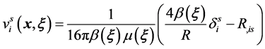
The system (4.3) at ν = const has Green’s function
 (4.4)
(4.4)
It is easy to be convinced of it. If to divide the equations of system (4.3) on μ, then we receive
 (4.5)
(4.5)
and then the solution (4.4) becomes obvious.
Remark. Expressions (2.11) and (4.4) formally match up, but between them there is the important difference. The formula (2.11) is the consequence of the assumption (2.10), and the formula (4.4) is the solution of system of equations.
Now for (4.1) by analogy with (2.5)-(2.8) it is possible to write the system of the integro-differential equations
 (4.6)
(4.6)
5. Some Data on Fourier’s Transformation
Let’s note some properties of Fourier’s transformation which will be used further. In this section and further we will designate Cartesian axials (x, y, z) and Fourier’s transformation by the sign “~” or by the arrow . We will determine direct and inversion Fourier’s transformations by formulas
 (5.1)
(5.1)
Transformation of the derivative on x leads to multiplication of the transform on .
.
We have some useful formulas. The Fourier’s transformation of product of functions is
 (5.2)
(5.2)
Differentiating the first formula (5.1) on p, we receive
 (5.3)
(5.3)
We have also formula
 (5.5)
(5.5)
We will determine Fourier’s double transformation by formulas
 (5.6)
(5.6)
In the axisymmetric case from (5.6) we receive Hankel’s transformation
 (5.7)
(5.7)
where ,
,  and
and  is the Bessel’s function.
6. Unidimensional Inhomogeneous Medium
Let’s consider unidimensional inhomogeneous on the axis z medium. Such problems matter in sciences of the Earth. Let’s designate displacements on axes (x, y, z) as (u, v, w). In these conditions of the balance equations in displacements has the kind
 (6.1)
(6.1)
where ,
,  and Δ is the Laplacian operator.
It is possible to apply the general methods stated in Sections 2 and 3 to the solution of system (6.1). However, it is better to make double Fourier’s transformation on (x, y) according to Section 5. Then (6.1) takes the form

(6.2)
Application of the general methods to (6.2) is more reasonable as in this case we receive system of the one-dimensional integro-differential equations. For the system
 (6.3)
(6.3)
with constant elastic moduli Green’s function is Calvin’s tensor (2.11) transformed by Fourier’s transformation.
As in Section 4, it is possible to investigate the case of constant coefficient of Poisson. In this case the system (6.2) can receive other form if to divide the Equations (6.2) on 

(6.4)
where  and
and .
.
7. Conclusion
Formulas (2.11) and (4.4) can be considered as zero-order approximation of Green’s function for the inhomogeneous medium. These formulas allocate part of the formula of Green with singularity. For the half-space it is necessary to apply Mindlin’s tensor [3] . It is possible to consider two-dimensional heterogeneity. In Section 6 it is possible to apply Fourier’s transformation on the final interval to finite bodies.
Cite this paper
Dobrovolsky, I.P. (2016) About the Integral Equations for Calculation of Green’s Tensor in Elastic Inhomogeneous Medium. Open Access Library Journal, 3: e3077. http://dx.doi.org/10.4236/oalib.1103077
References
- 1. Dobrovolsky, I.P. (2014) The Integral Equation, Corresponding to the Ordinary Differential Equation. Open Access Library Journal, 1, e1058.
http://dx.doi.org/10.4236/oalib.1101058 - 2. Dobrovolsky, I.P. (2015) Unidimensional Inhomogeneous Isotropic Elastic Half-Space. Open Access Library Journal, 2, e1670.
http://dx.doi.org/10.4236/oalib.1101670 - 3. Dobrovolskiy, I.P. (2013) Inhomogeneity and Inclusion in the Linear Elasticity Theory. Nauka i Studia. NR, 35, 49-58.