American Journal of Computational Mathematics, 2011, 1, 176-182
doi:10.4236/ajcm.2011.13020 Published Online September 2011 (http://www.SciRP.org/journal/ajcm)
Haar Wavelet Quasilinearization Approach for Solving
Nonlinear Boundary Value Pr oblems
Harpreet Kaur1, R. C. Mittal2, Vinod Mishra3
1,3Department of Mat hematics, Sant Longowal Institute of Engineering & Technology, Longowal, India
2Department of Mat hem at i cs, Indian Institute of Techn ology Roorkee, Roorkee, India
Received May 16, 2011; revised June 14, 2011; accepted June 26, 2011
Abstract
Objective of our paper is to present the Haar wavelet based solutions of boundary value problems by Haar
collocation method and utilizing Quasilinearization technique to resolve quadratic nonlinearity in y. More
accurate solutions are obtained by wavelet decomposition in the form of a multiresolution analysis of the
function which represents solution of boundary value problems. Through this analysis, solutions are found
on the coarse grid points and refined towards higher accuracy by increasing the level of the Haar wavelets. A
distinctive feature of the proposed method is its simplicity and applicability for a variety of boundary condi-
tions. Numerical tests are performed to check the applicability and efficiency. C++ program is developed to
find the wavelet solution.
Keywords: Haar Wavelets, Quasilinearization Technique, Haar Collocation Method, Boundary Value
Problems
1. Introduction
Wavelets are mathematical tools that cut up data, func-
tions or operators into different frequency components
and then study each component with a resolution match-
ing its scale. Much of the work on Haar functions was
performed in the 1930s. In 1909, Haar discovered the
simplest function now called as Haar wavelet. The inte-
gral of Haar family called Haar operational matrix was
derived by Chen and Hsiao [1] in 1997. Since then the
solutions of dynamical systems in a wavelet framework
took tremendous growth. In order to take the advantages
of the local property, many authors researched the Haar
wavelet to solve the linear stiff systems and differential
equations [2-4].
Haar function is a rectangular pulse pair. It is infact
the Daubechies wavelet of order one and is the simplest
of the orthonormal wavelets with compact support. As
shortcoming, Haar wavelets are not continuous; their
derivatives do not exist at the points of discontinuities.
Thereby direct application of Haar wavelet is not possi-
ble in solving differential equations but here one possi-
bility is through integration of wavelets [2]. The pro-
posed technique in this paper is based on collocation
framework and utilizes the capabilities of Haar wavelet
basis which permits to enlarge the class of functions
through Quasilinearization. Our main concentration on
the following type of nonlinear boundary value problems
defined in the interval [a, b].




1
,, ,,n
n
yt ftyyy

  (1)
subject to boundary conditions







 



12
1
3
12
1
3
,,
,,
,,
,,
nn
nn
yay a
yay a
yby b
yby b








 
 
 
 


f is a continuous function, in case of nonlinearity of f is at
most quadratic in y.
2. Preliminary Works
2.1. Haar Wavelets
Fourier transform analyzes the composition of a given
function in terms of sinusoidal waves of different fre-
quencies and amplitudes whereas wavelets analysis tells
how a given function changes from one time period to

H. KAUR ET AL.
177
the next. Wavelet analysis is also more flexible in sense
that one can choose a specific wavelet to match the type
of function being analyzed.
For a function , defined over the real axis

 

,


, is classed as a wavelet if it satisfies the following
three properties:


1) The integral of is zero:

 

d0tt 





 
2) The integral of the square of is unity:
is finite.

2dtt



3) Admissibility condition:

0
ˆdsatisfies 0.C

 



C 

The Haar scaling function for


0,1t is defined as

0
1if0 1
0elsewhere
t
ht 


 (2)
and corresponding wavelet function

1
1
1if0 2
1
1if0 2
0elsewhere
t
t
ht









(3)
Also the graph of is shown in Figure 1 [1].
The orthogonality property puts a strong limitation on
the construction of wavelets. It is known that the Haar
wavelet is the only real valued wavelet that is compactly
supported, symmetric and orthogonal. Thus Haar wave-
lets is orthogonal square waves family with mag-
nitude and zero, generally written as

i
ht
1

122
j
i
j
k
ht ht




for .
2,21,0, 021
j
ii kjk 
j
2.2. Multiresolution Analysis
Objective of this section is to construct a wavelet system,
which is complete orthonormal set in The idea
of multiresolution analysis is to represent a function f as

2
LR
1
1
0 0.5
–
1
t
h
1
(t)
Figure1. First haar wavelet.
a limit of successive approximations and decomposition
of the whole function space into individual subspaces
1
j
j
VV

. A multiresolution analysis (MRA) of


2
LR
is defined as a sequence of closed subspaces of
j
V of


2
LR, jZ

, that satisfy the following axioms:
1) Monotonicity
101
VVV

 
2) The spaces
j
V satisfy and

jz j
VLR
2jz j
V





0.
3)


0
f
tV

iff


2jj
f
tV jZ

 i.e. the space
j
V
are scaled versions of the central space .
0
V
4) There exists 0 V


s.t. is a Ri-
esz basis in .


,tkkZ  
0
The sequence
V




2jj 
,
jk kforms an
orthogonal basis for
22ttk  
j
V by using the multiresolution
analysis axioms. The space
j
V is used to approximate
general functions by defining appropriate projection of
these functions onto these spaces.
The vector space is the orthogonal complement
of
j
W
1jj
VV


. In other words, we will let be the
space of all functions in under the chosen inner
product. See [5] for detail of MRA. As an example the
space can be defined like
j
W
j
V
j
V
1112 2
0
1
1
,
jj jjjj
j
J
j
VW VW WV
WV
 




 

then the scaling function generates an MRA for
the sequence of spaces

1
ht


Z,
j
Vj by translation and
dilation as defined in (2) and (3). The linearly independ-
ent functions


,jk t
 spanning
j
W are called wavelets.
Original signal can be expressed as a linear combination
of the box basis functions in
j
V. These basis functions
have two important properties: orthogonality property
with






0,00,01,0 1,1
,,,ttt   t and normalization
of




2
,22, ,
jj
jk ttkj
 kZ

.
3. Haar Wavelet Integration and the
Quasilinearization Approach
The wavelets corresponding to the box basis are known
as the Haar wavelets.




1for ,
1for, ,
0 elsewhere
i
t
ht t
,






 



(4)
Here 0.5 1
,,,2,
j
kk k
m
mm m
 

 0,1,, .jJ


J indicates the level of resolution. The integer
0,1, ,k

 1m

is the translation parameter. The in-
dexing i in (4) is calculated as . In case with 1imk

178 H. KAUR ET AL.
minimal values . The maximal value
of i is
1,0, 2mk i
1
22
j
m .
Consider the collocation points 0.5 ,
2
ll
t
 
0d
t
ii
hxx
 
222
d
mm
m
hxxPh

m


0,1
1, 2l
22m
,,2.m
m

,1
Pt
0
t

The operational matrix P which is a
square matrix is defined by
(5)
Remarkable that [3] considers integral of Haar wave-
lets as
  
2
,
m
t t (6)
and operational matrix is
 

1
4
1,
40
mm mm
mm mm
mP H
mH








22 mm
P

But we have considered the integral of Haar wavelets
as following:
 



0
for ,
dfor
0elsewhere
t
ii
tt
hxx tt
,1
Pt ,












 
 

2
2
2
,2
i
Pt
2
1for ,
2
11 for ,
2
4
1for ,1
4
0elsewhere
tt
tt
m
t
m






 

t











th
n
We also introduce the following notation for specific
value of function

1
,1 ,1
0
d
ii
DPt
The Quasilinearization technique [6] is an application
of the Newton-Raphson-Kantrovich approximation me-
thod in function space. This method is applied to solve a
nonlinear order ordinary or partial differential equa-
tion in N-dimensions as a limit of a sequence of linear
differential equations. The idea of the method is based on
the fact that how to solve the nonlinear ODE’s by Haar
wavelets while there are no useful techniques for obtain-
ing the general solution of a nonlinear equation in terms
of a finite set of particular solutions. But we limit our-
selves here for variables according to involved variables
in nonlinear ordinary differential in the interval


, ,ab
.
0,a1b

 










123 1
,, ,,,,
nn
Lytfytyt ytytytt


with initial conditions

















12 1
12 1
,, ,,
,, ,,
n
n
hya yayaya
gyby bybyb


0
0




Here is the linear order ordinary differential
operator, f is nonlinear functions of

n
Lth n


y
t and its 1n

derivatives are


2,
j
yt,1,j,n1

 .
The Quasilinearization prescription determines the (r
+ 1)th iterative approximation

1r
y
t
 to the solution of
order nonlinear ordinary differential Equations (1)
as a solution of linear differential equation.
th
n














 







1
121
1
1
0
11
,,,, ,
,,,,,
j
nr
n
rr rr
njj
rr
j
n
rr r
y
Ly t
f
ytytytytt
yt yt
fytyty tt











where




0
rr
yt yt. The functions

j
j
y
f
fy



are
functional derivatives of the functional









121
,,,,,
n
fytyt ytytt
0


and


















12 1
12 1
11
,, ,,
,, ,,
n
n
rrr
hyay ayaya
gyby bybyb
ytytyt 



0.
0





The zeroth iteration


0
y
t is chosen as Haar wavelet
basis from physical and mathematical considerations of
given problem.
In [7] proved
 
2
1rr that showed
the difference between exact solution and the rth iteration
is decreasing quadratically and
yt kyt

1r
y
t 
 for an arbi-
trary lr

satisfied the following inequality:
 

1
2
1
r
rl
y
tkyt 

k
the Haar wavelet series considered as function approxi-
mation in Quasilinearization technique which satisfies
the boundary conditions of given problem. Then Qua-
silinearization procedure is adopted through Haar wave-
let collocation method for getting the solution of con-
cerning problems.
4. Error Analysis of Haar Wavelets
Let

and

are the scaling and the corresponding

H. KAUR ET AL.
179

wavelet function of respectively, also imply the
relations

2
LR

dtt 


d1, 0tt 

 

 (the moment properties).
The following dilation relation holds:
 
2thtl  

2
1
2
L
l
lL


12
,,L Z
(7)
with some and the family wavelets
hlR L




2
,
2
,
22 ,
22 ,,
jj
jk
jj
jk
ttk
ttkjk



 Z
j
P and
j
Q be the corresponding projections
1
,, ,,
,, ,,
,d
,d
jjj
jjkjkjkjk
jjkjkjkj
VVW
Pyccy t
Qyddy t






k
Let 21
M
MMp of the supports of wavelets

and

. M stands for th
M
moment of wavelet func-
tion. Then according to [8], we have the following theo-
rem:
Theorem. Assume the moment condition. For y


,
l
CR 1k,

 the following estimation holds:

2
max ,
j
l
jwt M
yPy Ayw jZ


 
where stands for derivative of y.

l
yw
Remark. For Haar function, .
Let be bounded first derivative on (0,1)
such that

12
1,0, 1MMM


2
yLR

l
yw SThen error at jth level will be given
by
22
kj kj
jj
yPyRSyPyA


A and R are suitable real constants.
5. Function Approximations
Orthogonality of Haar wavelets ensures that any square
integral function over [0, 1] can be expressed as an infi-
nite sum of Haar wavelets as

1
,
ii
i
f
taht



where ’s are wavelet coefficients.
i
a
If


f
t is piecewise constant or can be approxi-
mated as piecewise constant during each subinterval,
then sum can be terminated to finite term as [8]

1
2T
1
j
ii
i
ytahtaH




A function


2
f
LR is a MRA of


2
LR pro-
duces a sequence of subspaces
j
V of


2
LR, jZ

s.t. the projection of f onto these spaces give finer ap-
proximation of the function f as .
j
To demonstrate the applicability of Haar wavelets, we
focus on the following nonlinear BVP’s and utilizing
C++ Programming and MATLAB Software. In finite
element method the approximate solution can be written
as a linear combination of basis functions which consti-
tute a basis for the approximation space under considera-
tion.
Here in Haar collocation method the series is taken as
the highest derivative of given differential equation as a
linear combination of Haar wavelet basis.

 
1
2
1
j
nii
i
y
tah


t
Subsequent integrations give lower derivatives and


y
t. Substituting the values in the given equation gives
the coefficients and hence the solution.
6. Test Problems
6.1. Nonlinear Boundary Value Problems
6.1.1. Two Point Boundary Value Problem
Firstly, the application of Haar wavelets by Quasilin-
earization has been performed on the second order BVP
of purely mathematical nature [9] which posses analytic
solution and given by:
 
 
22 4
2πcos 2πsin π,
01,00and10.
yyttt
ty y
  
 (8)
with analytic solution


2
sin πyt t

. Approximate the
solution as


πsin
n
y
t
By wavelet based Quasilinearization technique,






2
2sin πsinπyttyt t

2
t
and Equation (8) be-
comes
 
 
21
224
2sin π2sinπ
sin π2πcos2πsin π.
aHtP ttP
tt
 

 
Efficiency of method for solution of second order
BVP problem is depicted in Figure 2, for j = 2 and j = 3.
6.1.2. Fourth Order Boundary Value Problem
Consider the fourth order nonlinear boundary value
problem [10]
210 9 8 7 64
''''4 448 412048,
01.
yyttttttt
t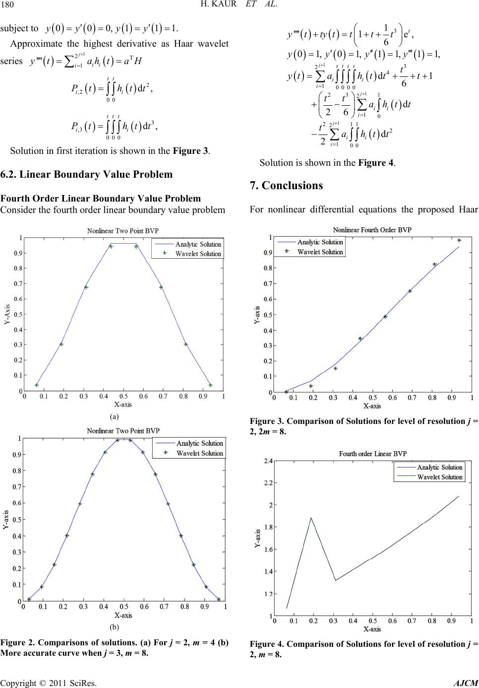
 


180 H. KAUR ET AL.
subject to



000,11yy yy

 
1.
Approximate the highest derivative as Haar wavelet
series
 
1
2T
1
''''
j
ii
i
ytaht aH




 
 
2
,2
00
3
,3
000
d,
d,
tt
ii
ttt
ii
Pt htt
Pt htt




Solution in first iteration is shown in the Figure 3.
6.2. Linear Boundary Value Problem
Fourth Order Linear Boundary Value Problem
Consider the fourth order linear boundary value problem
(a)
(b)
Figure 2. Comparisons of solutions. (a) For j = 2, m = 4 (b)
More accurate curve when j = 3, m = 8.
 
 
 


1
1
1
3
3
24
10000
1
23
2
10
11 222
100
1
''''1e ,
6
01,01, 11, 11
d1
6
d
26
d
2
j
j
j
t
tttt
ii
i
ii
i
ii
i
yttytttt
yy yy
t
ytah ttt
tt aht t
tahtt










 ,













Solution is shown in the Figure 4.
7. Conclusions
For nonlinear differential equations the proposed Haar
Figure 3. Comparison of Solutions for level of resolution j =
2, 2m = 8.
Figure 4. Comparison of Solutions for level of resolution j =
2, m = 8.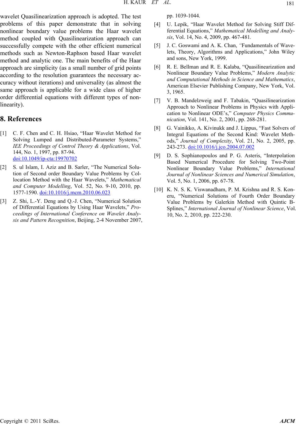

H. KAUR ET AL.
181
wavelet Quasilinearization approach is adopted. The test
problems of this paper demonstrate that in solving
nonlinear boundary value problems the Haar wavelet
method coupled with Quasilinearization approach can
successfully compete with the other efficient numerical
methods such as Newton-Raphson based Haar wavelet
method and analytic one. The main benefits of the Haar
approach are simplicity (as a small number of grid points
according to the resolution guarantees the necessary ac-
curacy without iterations) and universality (as almost the
same approach is applicable for a wide class of higher
order differential equations with different types of non-
linearity).
8. References
[1] C. F. Chen and C. H. Hsiao, “Haar Wavelet Method for
Solving Lumped and Distributed-Parameter Systems,”
IEE Proceedings of Control Theory & Applications, Vol.
144, No. 1, 1997, pp. 87-94.
doi:10.1049/ip-cta:19970702
[2] S. ul Islam, I. Aziz and B. Sarler, “The Numerical Solu-
tion of Second order Boundary Value Problems by Col-
location Method with the Haar Wavelets,” Mathematical
and Computer Modelling, Vol. 52, No. 9-10, 2010, pp.
1577-1590. doi:10.1016/j.mcm.2010.06.023
[3] Z. Shi, L.-Y. Deng and Q.-J. Chen, “Numerical Solution
of Differential Equations by Using Haar Wavelets,” Pro-
ceedings of International Conference on Wavelet Analy-
sis and Pattern Recognition, Beijing, 2-4 November 2007,
pp. 1039-1044.
[4] U. Lepik, “Haar Wavelet Method for Solving Stiff Dif-
ferential Equations,” Mathematical Modelling and Analy-
sis, Vol. 14, No. 4, 2009, pp. 467-481.
[5] J. C. Goswami and A. K. Chan, “Fundamentals of Wave-
lets, Theory, Algorithms and Applications,” John Wiley
and sons, New York, 1999.
[6] R. E. Bellman and R. E. Kalaba, “Quasilinearization and
Nonlinear Boundary Value Problems,” Modern Analytic
and Computational Methods in Science and Mathematics,
American Elsevier Publishing Company, New York, Vol.
3, 1965.
[7] V. B. Mandelzweig and F. Tabakin, “Quasilinearization
Approach to Nonlinear Problems in Physics with Appli-
cation to Nonlinear ODE’s,” Computer Physics Commu-
nication, Vol. 141, No. 2, 2001, pp. 268-281.
[8] G. Vainikko, A. Kivinukk and J. Lippus, “Fast Solvers of
Integral Equations of the Second Kind: Wavelet Meth-
ods,” Journal of Complexity, Vol. 21, No. 2, 2005, pp.
243-273. doi:10.1016/j.jco.2004.07.002
[9] D. S. Sophianopoulos and P. G. Asteris, “Interpolation
Based Numerical Procedure for Solving Two-Point
Nonlinear Boundary Value Problems,” International
Journal of Nonlinear Sciences and Numerical Simulation,
Vol. 5, No. 1, 2006, pp. 67-78.
[10] K. N. S. K. Viswanadham, P. M. Krishna and R. S. Kon-
eru, “Numerical Solutions of Fourth Order Boundary
Value Problems by Galerkin Method with Quintic B-
Splines,” International Journal of Nonlinear Science, Vol.
10, No. 2, 2010, pp. 222-230.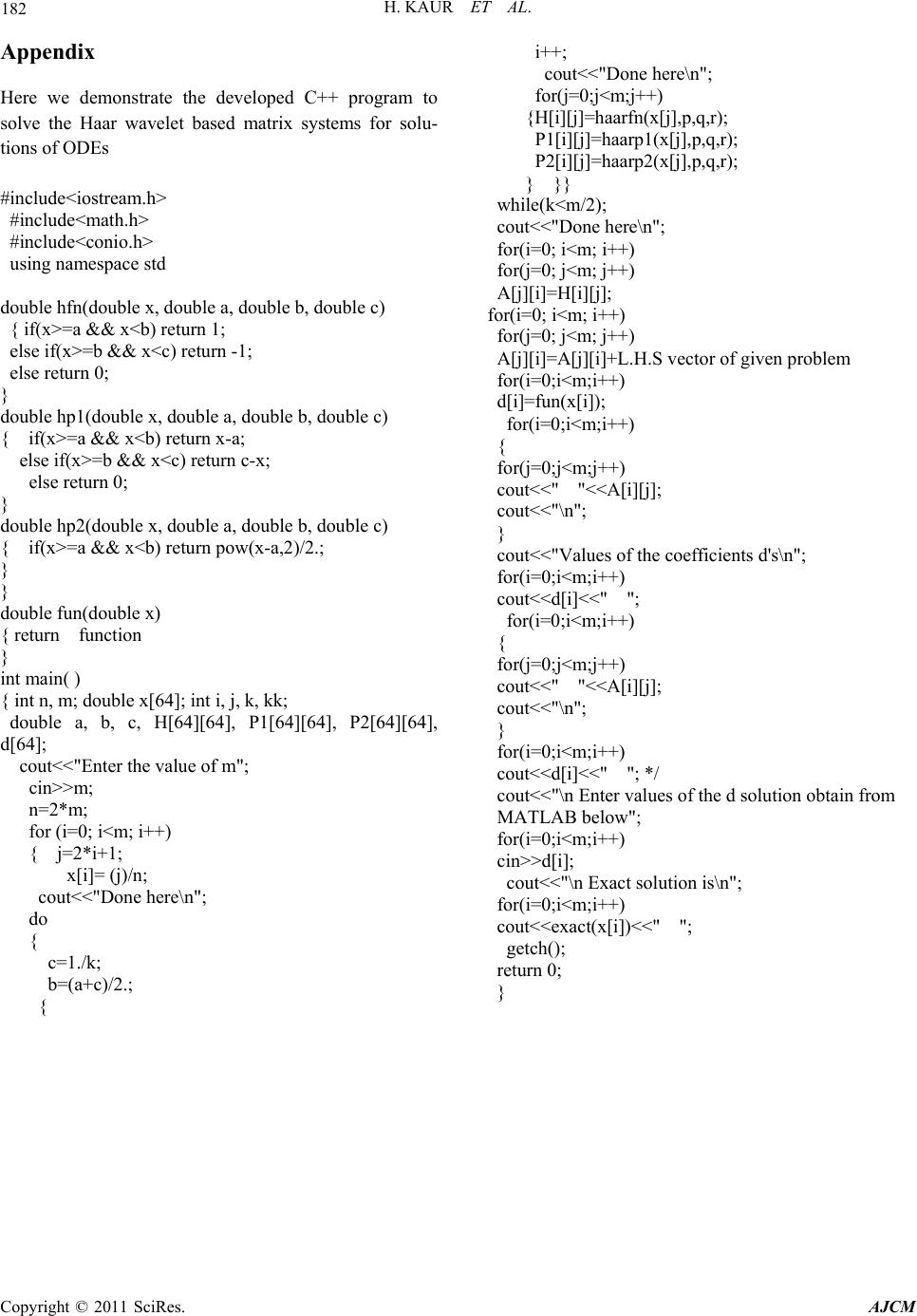

H. KAUR ET AL.
182
Appendix
Here we demonstrate the developed C++ program to
solve the Haar wavelet based matrix systems for solu-
tions of ODEs
#include<iostream.h>
#include<math.h>
#include<conio.h>
using namespace std
double hfn(double x, double a, double b, double c)
{ if(x>=a && x<b) return 1;
else if(x>=b && x<c) return -1;
else return 0;
}
double hp1(double x, double a, double b, double c)
{ if(x>=a && x<b) return x-a;
else if(x>=b && x<c) return c-x;
else return 0;
}
double hp2(double x, double a, double b, double c)
{ if(x>=a && x<b) return pow(x-a,2)/2.;
}
}
double fun(double x)
{ return function
}
int main( )
{ int n, m; double x[64]; int i, j, k, kk;
double a, b, c, H[64][64], P1[64][64], P2[64][64],
d[64];
cout<<"Enter the value of m";
cin>>m;
n=2*m;
for (i=0; i<m; i++)
{ j=2*i+1;
x[i]= (j)/n;
cout<<"Done here\n";
do
{
c=1./k;
b=(a+c)/2.;
{
i++;
cout<<"Done here\n";
for(j=0;j<m;j++)
{H[i][j]=haarfn(x[j],p,q,r);
P1[i][j]=haarp1(x[j],p,q,r);
P2[i][j]=haarp2(x[j],p,q,r);
} }}
while(k<m/2);
cout<<"Done here\n";
for(i=0; i<m; i++)
for(j=0; j<m; j++)
A[j][i]=H[i][j];
for(i=0; i<m; i++)
for(j=0; j<m; j++)
A[j][i]=A[j][i]+L.H.S vector of given problem
for(i=0;i<m;i++)
d[i]=fun(x[i]);
for(i=0;i<m;i++)
{
for(j=0;j<m;j++)
cout<<" "<<A[i][j];
cout<<"\n";
}
cout<<"Values of the coefficients d's\n";
for(i=0;i<m;i++)
cout<<d[i]<<" ";
for(i=0;i<m;i++)
{
for(j=0;j<m;j++)
cout<<" "<<A[i][j];
cout<<"\n";
}
for(i=0;i<m;i++)
cout<<d[i]<<" "; */
cout<<"\n Enter values of the d solution obtain from
MATLAB below";
for(i=0;i<m;i++)
cin>>d[i];
cout<<"\n Exact solution is\n";
for(i=0;i<m;i++)
cout<<exact(x[i])<<" ";
getch();
return 0;
}