American Journal of Computational Mathematics, 2011, 1, 159-162
doi:10.4236/ajcm.2011.13018 Published Online September 2011 (http://www.SciRP.org/journal/ajcm)
Quasi-Reversibility Regularization Method for Solving a
Backward Heat Conduction Problem
Ailin Qian*, Jianfeng Mao
School of Mathematics and Statistics, Xianning University, Xianning, China
Received July 15, 2011; revised August 22, 2011; accepted September 2, 2011
Abstract
Non-standard backward heat conduction problem is ill-posed in the sense that the solution (if it exists) does
not depend continuously on the data. In this paper, we propose a regularization strategy-quasi-reversibility
method to analysis the stability of the problem. Meanwhile, we investigate the roles of regularization pa-
rameter in this method. Numerical result shows that our algorithm is effective and stable.
Keywords: Back Heat Conduction, Ill-Posed Problem, Quasi-Reversibility, Regularization
1. Introduction
In many industrial application one wishes to determine
the temperature on the surface of a body, where the sur-
face itself is inaccessible for measurement. The back-
ward heat conduction problem is a model of this situation.
In general, no solution which satisfies the heat conduc-
tion equation with final data and the boundary conditions
exists. Even if a solution exists, it will not be continu-
ously dependent on the final data. The BHCP is a typical
example of an ill-posed problem which is unstable by
numerical methods and requires special regularization
methods. In the context of approximation method for this
problem, many approaches have been investigated. Such
authors as Lattes and Lions [1], Showalter [2], Ames et
al. [3], Miller [4] have approximated the BHCP by quasi-
reversibility methods. Schröter and Tautenhahn [5] es-
tablished an optimal error estimate for a special BHCP.
Mera and Jourhmane used many numerical methods with
regularization techniques to approximate the problem in
[6-8], etc. A mollification method has been studied by
Haö in [9]. Kirkup and Wadsworth used an operator-
splitting method in [10]. So far in the literature, most of
the authors used the eigenfunctions and eigenvalues to
reconstruct the solution of the BHCP by many quasi-
reversibility methods numerically. However, the eigen-
functions and eigenvalues are in general not available
and the labor needed to compute these and the corre-
sponding fourier coefficients is very onerous. In this pa-
per, we use a quasi-reversibility regularization method to
solve the BHCP in one-dimensional setting numerically,
but this method can be generalized to two-dimensional
case.
The paper is organized as follows. In the forthcoming
section, we will present the mathematical problem on a
BHCP; in Section 2, we review a special quasi-reversi-
bility regularization method; some finite difference
schemes are constructed for the inverse problem and the
numerical stability analysis is provided; in Section 3,
numerical example is tested to verify the effect of the
numerical schemes.
2. Mathematical Problem
2.1. The Direct Problem
We consider the following heat equation:






 

 
,,=,,π<<π,0< <,
π,=, 0<<,
π,=, 0<<,
,0=, π<<π.
tx xx
uxtuxtuxtxt T
utst tT
utlt tT
uxf xx




(1)
Solving the equation with given
 


,,
s
tlt fx is
called a direct problem. From the theory of heat equation,
we can see that for


,,

s
tlt fx in some function
space there exists a unique solution [11-20].
2.2. The Inverse Problem
Consider the following problem:






,,=,,π<<π, 0<<,
tx xx
uxtuxtuxtxt T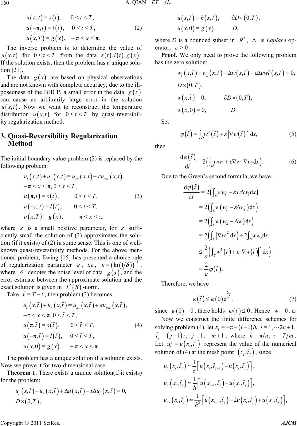

160 A. QIAN ET AL.
 

 
π,=, 0<<,
π,=, 0<<,
,=, π<<π.
utst tT
utlt tT
uxT gxx


(2)
The inverse problem is to determine the value of
for from the data

,uxt 0<tT





,,
s
tltgx.
If the solution exists, then the problem has a unique solu-
tion [21].
The data

g
x are based on physical observations
and are not known with complete accuracy, due to the ill-
posedness of the BHCP, a small error in the data


g
x
can cause an arbitrarily large error in the solution
. Now we want to reconstruct the temperature
distribution for by quasi-reversibil-
ity regularization method.

,uxt

,uxt

0<tT
3. Quasi-Reversibility Regularization
Method
The initial boundary value problem (2) is replaced by the
following problem:
 
 

 
,,=, ,
π<<π,0< <,
π,=, 0<<,
π,=, 0<<,
,=, π<<π.
t xxxxxt
u xtuxtuxtuxt
xtT
utst tT
utlt tT
uxT gxx
 



,
(3)
where

is a small positive parameter, for

suffi-
ciently small the solution of (3) approximates the solu-
tion (if it exists) of (2) in some sense. This is one of well-
known quasi-reversibility methods. For the above men-
tioned problem, Ewing [15] has presented a choice rule
of regularization parameter

, i.e. ,
 
1
=ln1 

,
where

denotes the noise level of data

g
x, and the
error estimate between the approximate solution and the
exact solution is given in


2
LR-norm.
Take , then problem (3) becomes =tTt

 


 
,,=, ,
π<<π,0<<,
π,=, 0<<,
π,=, 0<<,
,0=, π<<π.
xxx t xxt
uxtuxtu xtuxt
xtT
ut sttT
utlt tT
ux gxx
 




 

 
 
,

=0,
(4)
The problem has a unique solution if a solution exists.
Now we prove it for two-dimensional case.
Theorem 1. There exists a unique solution(if it exists)
for the problem:
 

,, ,,
0, ,
x tt
uxtuxtu xtuxt
DT
 


 



 
 
,=,, 0,,
,0=, .
uxthxtDT
ux gxD


where D is a bounded subset in , is Laplace op-
erator,
2
R
>0

.
Proof. We only need to prove the following problem
has the zero solution:










,, ,,
0, ,
,=0,0,,
,0= 0,.
x t
wxtwxtwxtuwtxt
DT
wxtD T
wx D
 


 

=0,
Set
 
2
2
=d
D
twtwt  

 
,x
(5)
then



d=2d .
dtt
D
twwww x
t

 


 (6)
Due to the Green’s second formula, we have








 


2
2
2
d=2 d
d
= 2d
= 2d
=2d2d
2
d
2
=.
tt
D
tt
D
x
D
x
DD
D
twww wx
t
wwwx
www x
wx wwx
wtwt x
t






















Therefore, we have


2
0e .
t
t

 
 (7)
since


0=0  , there holds , Hence . □

0t  
=0w
Now we construct the finite difference schemes for
solving problem (4), let


=π1,
i
x
ih  =1, 21,in




=1
j
tj,


 =1,j1m

, where =π,=hn Tm

.
Let


,
i j
xt

=
j
i
uu represent the value of the numerical
solution of (4) at the mesh point

,
ij
x
t
, since
 
 
 
1
1
1
2
1
,,,,
1
,,,,
1
,,2,
ijij ij t
xiji jij
xx ijijijij
uxtuxt uxt
uxtux tuxt
h
uxtuxtuxt uxt
h










,,













A. QIAN ET AL.
161
 


11 1
2
1
11 1
11
,,
2
,,
1
,,.
ijij ij xxt
ij ij
ij ij
uxtuxt uxt
h
uxt uxt
ux tuxt



 


















,



then Equation (4) is discretized as
111
11
1
22
1
2
1
2
112 11
=2
1
.
jjj
iii
j
j
ii
i
ruru ru
rur u
hh
hh
h







 


 
 
 
 

(8)
where
j
ru



2
=, =2,,2, =1,,.ri nj
h


 m
Now we discuss the stability of difference sch
by verifying the Von Neumann condition. The propaga-
tion factor can be found
emes (8)

2
2
2
11
4sin 2
,= .
14sin 2
r
h
r
h
Gh


 





(9)

It is easy to verify the fact that Von Neumann condition

,1Gc.

  (10)
holds with =1c

, hence,the numerical algorithm
stable.
4. Numerical Examples
For convenience, we take
Example 1.We considerect problem:
(11)
w
(12)
Let
(8) is
 
=stlt
r the following di

=0 in (2).
 
,,=,, π<<π, 0<<1,
t
uxt 


π,= 0, 0<<1,
,
x xx
uxtu xtxt
ut t


π,=
0, 0<<1ut t
ith the initial condition:

π,π0,
,0 =π,0 π.
xx
ux xx




1=π,x


=π1,
i
x
ih 

=1,
=1,2,,2 ,in
21
=
n
xπ, j
tj

 =1,2, ,1, the spjm ace
step length =πhn, and the time step length =1 m

,
then we solve this problem by an ex



plicit differe
scheme in the following form:
nce

21 , 1
11
0, 0<<1,
,==0, 0<<1,
1
11
22
2
22
2
=1
22
=1, ,,=2, ,2,
==
j
2
,
jj
iii
j
t
j
hh
uuu
hhh
m n
u


j
i
u

nn
j
j
ji
ux t
uxt ut


)





 (13
with

1
π,π0,
,=0=
π,0π.
ii
iii
xx
uxt xx

 


 (14)
where 2
=rh  ,and it requires <1 2r for nume
stability reasons.
The numerical results for is sh-
own in Figure 1, where
w we solve the inverse problem by the
rical
 
=,=1gx uxT
11, =50nm . =
No


g
x
a the quasi-
gen-
numerical by the direct problem vi
reversibility regularization method. We ch
the solution
erated
oose to restore


f
x
e inv
at We denotes therical
h
=0t. e num
results of terse problem as


*
f
x. If we introduce
random noises

to data

g
x, i.e.,






=
ii
g
xgxrandi

 , wa ran-
dom number between [−e ise
h
], t
ere rand
hen th

is
tal no
i
to1, 1

can be measured in the sense of root mean s
according to:
quare error
  
21 2
1
1.
n
ii
i
gx gx
n






In the computation, we cse the regularization pa-
ram
21
hoo
eters


1
=ln1,=0.001 
, merical re-
sults are shown in Figure 2, where =11, = 50nm.
From Example, we conclude that the choice rules of
the regularization parameter
h  the nu

is very effective. By our
numerical experiment, we can see that the accuracy of
the numerical results increases with the decreasing T; at
Figure 1. g(x) computed by (13).

A. QIAN ET AL.
162
doi:10.1080/10682760290004320
[8] N. S. Mera, “The Method of Fundamental Solutions for
the Backward Heat Conduction Problem,” Inverse Pro b-
lems in Engineering, Vol. 13, No. 1, 2005, pp. 79-98.
doi:10.1080/10682760410001710141
[9] D. N. Haö, “A Mollification Method for Ill-Posed Prob-
lems,” Numerische Mathematik, Vol. 68, No. 4, 1994, pp.
469-506. doi:10.1007/s002110050073
[10] S. M. Kirkup and M. Wadsworth, “Solution of Inverse
Diffusion Problems by Operator-Splitting Methods,” Ap-
plied Mathematical Modelling, Vol. 26, No. 10, 2002, pp.
1003-1018. doi:10.1016/S0307-904X(02)00053-7
[11] C. L. Fu, X. T. Xiong and Z. Qian, “Fourier Regulariza-
tion for a Backward Heat Equation,” Journal of Mathe-
matical Analysis and Applications, Vol. 33, No. 1, 2007,
pp. 472-481. doi:10.1016/j.jmaa.2006.08.040
[12] L. Elden, “Numerical Solutiono of the Sideways Heat
Equation by Diference Approximation in Time,” Inverse
Problems, Vol. 201, No. 11, 1995, pp. 913-923.
doi:10.1088/0266-5611/11/4/017
Figur .145.
the same time, the numerical solutions of the quasi-re-
versibility method depend on the parameter
e 2. f* and f, m = 50, n = 11, ε = 0
[13] H. Han, D. B. Ingham and Y. Yuan, “The Boundary Ele-
ment Method for the Solution of the Backward Heat
Conduction Equation,” Journal of Computational Physics,
Vol. 116, No. 2, 1995, pp. 92-99.

co
tinuously. This accords with the theoretical result.
5. References
[1] R. Latter and J. L. Lions, “Methode de Quasi-Reversibil-
ity et Applications,” Dunod, Paris,1967.
[2] R. E. Showalter, “The Final Value Problem for Evolution
Equations,” Journal of Mathematical Analysis and Ap-
plications, Vol. 47, 1974, pp. 563-572.
doi:10.1016/0022-247X(74)90008-0
n-
doi:10.1006/jcph.1995.1028
[14] M. Jourhmane and N. S. Mera, “An Iterative Algorithm
for the Backward Heat Conduction Problem Based on
Variable Relaxtion Factors,” Inverse Problems in
l. 6, 1975,
Engneering, Vol. 10, No. 2, 2002, pp. 93-308.
[15] R. E. Ewing, “The Approximation of Cetain Parabolic
Equations Backward in Time by Sobolev Equations,”
SIAM Journal on Mathematical Analysis, Vo
[3] K. A. Ames, W. C. Gordon, J. F. Epperson and S. F.
penhermer, “A Comparison of Regularizations for an
Ill-Posed Problem,” Mathematics of Computation, Vol
67
do
pp. 283-294. doi:10.1137/0506029
[16] D. N. Hào and P. M. Hien, “Stability Results for the
Cauchy Problem for the Laplace Equation in a S
verse Problems, Vol. 19, No. 4, 2003, pp
Op-
. trip,” In-
. 833-844.
, No. 224, 1998, pp. 1451-1471.
i:10.1090/S0025-5718-98-01014-X [17] D. N. Hào and D. Lesnic, “The Cauchy for Laplace’s
Equation via the Conjugate Gradient Method,” IMA
Journal of Applied Mathematics, Vol. 65, 2000, pp. 199-
217. doi:10.1093/imamat/65.2.199
[4] K. Miller, “Stabilized Quasireversibility and Other
Nearly Best Possible Methods for Non-Well-Posed Prob-
lems,” Symposium on Non-Well-Posed Problems and
Logarithmic Convexity, Lecture Notes in Mathematics,
Springer-Verlag, Berlin, Vol. 316, 1973, pp. 161-176.
d U. Tautenhahn, “On Optimal Regulariza-
tion Methods for the Backward Heat Equation,”
on Problem,” In-
s Transfer, Vo
se Problems in
308.
[18] Y. C. Hon and T. Wei, “Backus-Gilbert Algorithm for the
Cauchy Problem of Laplace Equation,” Inverse Problems,
Vol. 17, 2001, pp. 261-271.
doi:10.1088/0266-5611/17/2/306
[5] T. Schröter an
Zeitschrift für Analysis und ihre Anwendungen, Vol. 15,
1996, pp. 475-493. [19] M. V. Klibanov and F. Santosa, “A Computational Quasi-
Reversibility Method for Cauchy Problems for Laplace’s
Equation,” SIAM Journal on Mathematical Analysis, Vol.
51, No. 6, 1991, pp. 1653-1675.
doi:10.1137/0151085
[6] N. S. Mera, L. Elliott, D. B. Ingham and D. Lesnic, “An
Iterative Boundary Element Method for Solving the One
Dimensional Backward Heat Conducti
ternational Journal of Heat and Masl. 44, [20] J. R. Cannon, “The One-Dimensional Heat Equation,”
Addison-Wesley Publishing Company, Menlo Park, 1984.
2001, pp. 1946-1973.
[7] M. Jourhmane and N. S. Mera, “An Iterative Algorithm
for the Backward Heat Conduction Problem Based on
Variable Relaxtion Factors,” Inver
neering, Vol. 10, No. 4, 2002, pp. 293-
[21] L. C. Evans, “Partial Differential Equations,” American
Mathematical Society, Providence, 1998.
Engi-
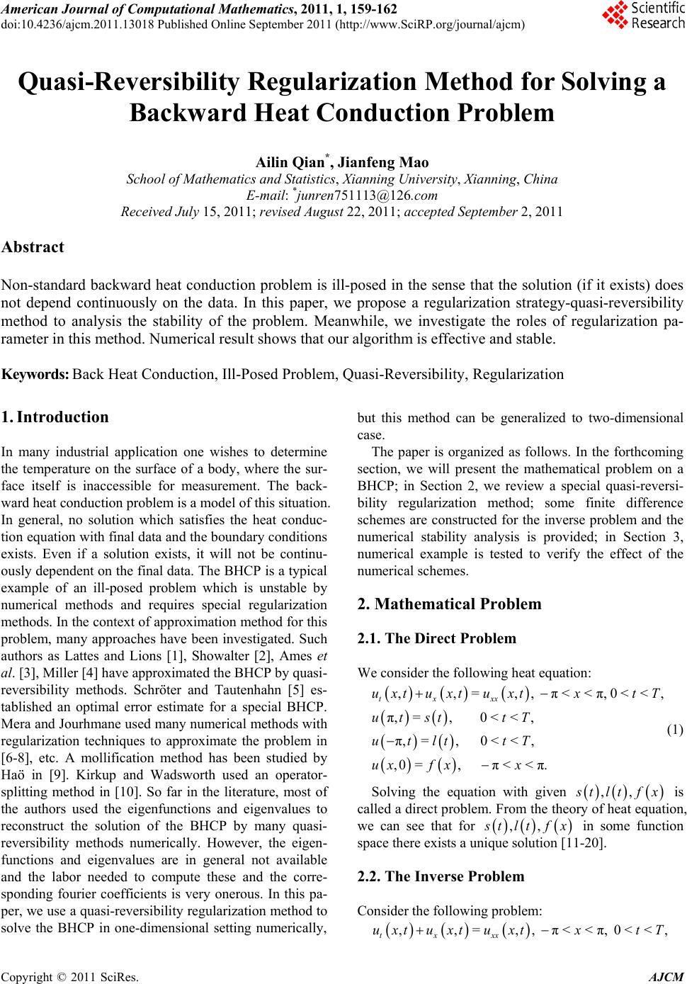