Journal of Signal and Information Processing, 2011, 2, 152-158
doi:10.4236/jsip.2011.23019 Published Online August 2011 (http://www.SciRP.org/journal/jsip)
RLS Wiener Predictor with Uncertain
Observations in Linear Discrete-Time Stochastic
Systems
Seiichi Nakamori1, Raquel Caballero-Águila2, Aurora Hermoso-Carazo3, Josefa Linares-Pérez3
1Department of Technical Education, Kagoshima University, Kagoshima, Japan; 2Departamento de Estadística e I.O, Universidad de
Jaén, Paraje Las Lagunillas, Jaén, Spain; 3Departamento de Estadística e I.O, Universidad de Granada, Campus Fuentenueva S/N,
Granada, Spain.
Received June 27th, 2011; revised July 29th, 2011; accepted August 8th, 2011.
ABSTRACT
This paper proposes recursive least-squares (RLS) l-step ahead predictor and filtering algorithms with uncertain ob-
servations in linear discrete-time stochastic systems. The observation equation is given by
 




y
kkzkv  k

,
, where is a binary switching sequence with cond itional probability. The estimators req uire the
information of the system state-transition matrix
 
zk Hxk


k 

, the observation matrix
H
, the variance

,
K
kk of the state
vector

x
k, the varia nce


Rk of the observation noise, the probability






1pk Pk 

 that the signal exists
in the uncertain observation equation and the


2, 2 element


2,
|Pk j2



 of the conditional probability of


k  ,
given .

j 
Keywords: Estimation Theory, Synthe sis of Stochastic Sy stems, RLS Wiener Predic tor, Uncertain Observations, Markov
Probability
1. Introduction
The estimation problem given uncertain observations is
an important research topic in the area of detection and
estimation problems in communication systems [1]. Nahi
[2], assuming that the state-space model is given, pro-
poses the RLS estimation method with uncertain obser-
vations, when the uncertainty is modeled in terms of in-
dependent random variables, and the probability that the
signal exists in each observation is available. The term
uncertain observations refers to the fact that some obser-
vations may not contain the signal and consist only of
observation noise. In Hadidi and Schwartz [3], Nahi’s
results are extended to the case where the variables mod-
eling the uncertainty are not necessarily independent.
In the above studies, it is assumed that the state-space
model for the signal is given. However, in real applica-
tions, the state-space modeling errors might degrade the
estimation accuracy. Nakamori [4] derived the RLS
Wiener fixed-point smoothing and filtering algorithms,
based on the invariant imbedding method, from uncertain
observations with uncertainty modeled by independent
random variables. In the derivation of such RLS Wiener
estimators, the state-transition matrix Φ, the observation
matrix
H
, the variance

,

K
kk of the state vector


x
k, the variance


Rk of the observation noise


vk and the observed values

y
k are used. More-
over, Nakamori et al. [5], based on the innovation ap-
proach, proposed the RLS Wiener fixed-point smoother
and filter in linear discrete-time stochastic systems. Here,
the observation equation is given by








y
kkzkv  k
 
zk Hxk, ,where




k 
is a binary switching sequence with conditional probabil-
ity. The innovation process is given by



 
ˆ,1,sysyss 






2,2
ˆˆ ,1 1sPsH xs

,1ys s




in terms of the element ,2 of the
conditional probability of , given
(2,2)

2
|Pk j

() j

k 

(see Na-
kamori et al. [5,6] for details).
In the current paper, under the same assumptions for
the observation equation as in Nakamori et al. [5], an
algorithm for the RLS Wiener ahead predictor
is derived, based on the invariant imbedding method.
Thus, the observation equation is given by
stepl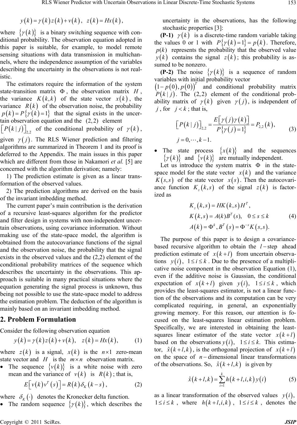

RLS Wiener Predictor with Uncertain Observations in Linear Discrete-Time Stochastic Systems153
 
y
kkzkvk

, ,
 
zk Hxk
where is a binary switching sequence with con-
ditional probability. The observation equation adopted in
this paper is suitable, for example, to model remote
sensing situations with data transmission in multichan-
nels, where the independence assumption of the variables
describing the uncertainty in the observations is not real-
istic.
 
k 

The estimators require the information of the system
state-transition matrix , the observation matrix

H
,
the variance

,

K
kk of the state vector


x
k, the
variance of the observation noise, the probability
that the signal exists in the uncer-
tain observation equation and the element

Rk
P
 

 
1k

pk

(2,2)

2,2
|Pk j 
 
of the conditional probability of


k  ,
given


j  . The RLS Wiener prediction and filtering
algorithms are summarized in Theorem 1 and its proof is
deferred to the Appendix. The main issues in this paper
which are different from those in Nakamori et al. [5] are
concerned with the algorithm derivation; namely:
1) The prediction estimate is given as a linear trans-
formation of the observed values.
2) The prediction algorithms are derived on the basis
of the invariant imbedding method.
The current paper’s main contribution is the derivation
of a recursive least-squares algorithm for the predictor
and filter design in systems with non-independent uncer-
tain observations, using covariance information. Without
making use of the state-space model, the algorithm is
obtained from the autocovariance functions of the signal
and the observation noise, the probability that the signal
exists in the observed values and the (2,2) element of the
conditional probability matrices of the sequence which
describes the uncertainty in the observations. This ap-
proach is suitable in many practical situations where the
equation generating the signal process is unknown, thus
being not possible to use the state-space model to address
the estimation problem. The deduction of the algorithm is
mainly based on an invariant imbedding method.
2. Problem Formulation
Consider the following observation equation
 
,,
y
kkzk vkzkHxk

  (1)
where is a signal,

zk

x
k is the zero-mean
state vector and
1n
H
is the mn

observation matrix.
 The sequence



vk is a white noise with zero
mean and the variance of


vk is

Rk; that is,
 
K
EvkvsRkks 



T
, (2)
where denotes the Kronecker delta function.

K
 
 The random sequence

 
k  , which describes the
uncertainty in the observations, has the following
stochastic properties [3]:
(P-1)


k  is a discrete-time random variable taking
the values 0 or 1 with


 
1
P
kp   k. Therefore,
represents the probability that the observed value ()pk


y
k contains the signal ; this probability is as-
sumed to be nonzero.

zk
(P-2) The noise




k 

is a sequence of random
variables with initial probability vector
and conditional probability matrix
 

10,0
T
pp


|Pk j(2,. The element of the conditional prob-
ability matrix of
2)


k  given


j  , is independent of
, for
jjk

; that is,
 
 

2,2
2,2
|,
1
0, ,1.
Ejk
Pk jPk
Pj
jk





 

(3)
 The state process



x
k and the sequences




k  and




vk are mutually independent.
Let us introduce the system matrix in the state-
space model for the state vector


x
k and the variance


,
K
ss of the state vector

x
s. Then the autocovari-
ance function


,
z
K
ks of the signal is factor-
ized as

zk




 
,,,
,()(),0
,,
T
z
T
kT s
Kks HKksH
.
K
ksAkB ssk
A
kBsKs


s


 
(4)
The purpose of this paper is to design a covariance-
based recursive algorithm to obtain the ahead
prediction estimate of
stepl


x
kl

from uncertain observa-
tions


y
i, 1ik

. Due to the presence of a multipli-
cative noise component in the observation Equation (1),
even if the additive noise is Gaussian, the conditional
expectation of


x
kl

given

,
y
i , which
provides the least-squares estimator, is not a linear func-
tion of the observations and its computation can be very
complicated requiring, in general, an exponentially
growing memory. For this reason, our attention is fo-
cused on the least-squares linear estimation problem.
Specifically, we are interested in obtaining the least-
squares linear estimator of the state vector
1ik


x
kl

based on the observations

,
y
i This estima-
tor,
1i.k


ˆ,
x
klk
, is the orthogonal projection of


x
kl

on the space of n

dimensional linear transformations
of the observations. So,


ˆ,
x
klk
is given by
 
1
ˆ,,,
k
i

x
klkhklikyi

 
 (5)
as a linear transformation of the observed values


,
y
i
1ik

, where


,,hklik, , denotes the 1ik

RLS Wiener Predictor with Uncertain Observations in Linear Discrete-Time Stochastic Systems 154
impulse-response function.
Let us consider the least-squares prediction problem,
which minimizes the criterion
     
ˆˆ ,,
T
JExklxk lkxk lxk lk

 

.


(6)
The orthogonal projection lemma [7] assures that

,
x
klk is the only linear combination of the obser-
vations


y
i, such that the estimation error is
orthogonal to them,
1ik
 
ˆ,, 1,
x
kl xklkyssk (7)
that is,
 
1
,,0,
1.
kT
i
Exk lhklikyiys
sk



 
 







This condition is equivalent to the Wiener–Hopf equa-
tion
  
1
,,,
1,
k
TT
i
Exk lyshklikEyiys
sk

 

 

 (8)
useful to determine the optimum impulse-response func-
tion


,,hklik, , which minimizes the cost
function (6). From , the left-hand
side of (7) is written as
1ik
Pk 



1pk



,
TT
Exk lysKklsHps




. (9)
Let


E



denote the statistical expectation with re-
spect to



vk
. Then, from the observation equation (1)
and the covariance function (2) for white observation
noise , is reduced to

T
Eyiy s

 
T
 
 
,
.
T
K
EyiysEis HKisH
Rii s







 (10)
Substituting (9) and (10) into (8), we have


1
,, ,
,,, .
T
kT
i
hk lskRsKk lsHps
hklikEisHK is H




 

 (11)
Under these conditions, in Section 3 the RLS Wiener
prediction and filtering algorithms are presented.
3. RLS Wiener Prediction and Filtering
Algorithm
Nakamori et al. [5,6], based on the innovation approach,
proposed the algorithms for the fixed-point smoothing
estimate and the filtering estimate. These algorithms are
derived taking into account that the innovation process is
expressed as







2,2
ˆ,1,
ˆˆ ,1 1,1
sysyss
yssPsH xss
  

.


Under the preliminary assumptions made in Section 2,
Theorem 1 proposes the RLS Wiener algorithms for the
stepl

ahead prediction estimates of the signal


zk l

and the state vector

x
kl. These algo-
rithms are derived, starting with (11), by iterative use of
the invariant imbedding method.
Theorem 1. Consider the observation equation de-
scribed in (1) and assume that the probability


pk and
the element (2,2)


2,2
Pk of the conditional probabil-
ity matrix


,
|Pk j are given. Let the system state-
transition matrix

the observation matrix ,
H
the
autovariance function


,
K
ss of the state vector


x
s,
the variance


Rk of the white observation noise


vk and the observed value

y
k
l
be given. Then the
RLS Wiener algorithms for the ahead predic-
tion estimate
step


, lk ˆ zk of the signal and the

zk

l
l

step ahead prediction estimate

,
ˆ
x
klk of the
state vector


x
kl

consist of (12)-(17).
l

step ahead prediction estimate of the signal




ˆ
:,lzk lkzk


ˆ ˆ,zk lkHxk lk 

, (12)
l

step ahead prediction estimate of the state vector




ˆ
:,
x
klxklk







2,2
ˆˆ ,1,1
ˆ
,,1,1,
ˆ,0 0
l
xk lkxk lk
hkkkykPkH xkk
xl

 

(13)
Filtering estimate of

 
ˆ
:,zk zkk


ˆ
ˆ,zkk Hxkk

, (14)
Filtering estimate of




ˆ :,
x
kxkk







2,2
ˆˆ ,1,1
ˆ ,,1,1,
ˆ0,00
xkkxk k
hkkkykPkHxkk
x



 (15)
Filter gain:


,,hkkk





 

 

 

2,2
1
2
2,2
,, ,
1
,
1
T
TT
T
TT
hkkkKkkH pk
PkSk H
Rk pkHKkkH
PkHSk H





(16)

RLS Wiener Predictor with Uncertain Observations in Linear Discrete-Time Stochastic Systems155
 


 


2,2
1,,
,1
00
T
T
Sk Skhkkk
HKkkpkPkHSk
S
 


, (17)
Proof of Theorem 1 is detailed in the Appendix.
Clearly, the algorithms for the filtering estimate are the
same as those proposed in Nakamori et al. [5]. From
Theorem 1, the innovation process


k  is represented
by
 
2,2 ˆ1,1 .kykPkHxkk
   (18)
4. A Numerical Simulation Example
In order to illustrate the application of the RLS Wiener
prediction algorithm proposed in Theorem 1, we consider
a scalar signal


zk whose autocovariance function

z
K
m

is given as follows [8]

 
 

 

2
22
1212 121
2
2122121
0,
11
11
0,
z
m
z
m
K
Km
m
,

 
 

  

 



(19)
with

2
12112
,4aaa   2,
where and
1 2
0.1,a 0.8a0.5.


The covariance function (19) corresponds to a signal
process generated by a second-order AR model. There-
fore, according to Nakamori [4], the observation vector
,
H
the variance of the state vector
 
,Kkk K

0

x
k and the system matrix in the state equation
are as follows:





 
 
21
01
10, ,,
10
01
,00.25,1 0.125.
zz
zz
zz
KK
HKkk
KK
KK
aa





 



(20)
As in Nakamori et al. [5], we consider that the signal
is transmitted through one of two channels, char-
acterized by its observation equation as follows:

zk
Channel 1:






,
y
kzkvk
 
Channel 2:


,
y
kUkzkvk

where is a zero-mean white observation noise
and is a sequence of independent random
variables taking values or 1 with


vk


Uk
0
 
1PU kp
0.8
.7
is described by
, for all . k
We assume that channel 1 is chosen at random with
probability and, hence, channel 2 is selected
with probability . Then, the observation equation
10q
0.3q






,
y
kkzkvk   (21)
where




11k   

Uk
and

is a random
variable, independent of



, taki values 0 or 1
with
Uk ng


10.3Pq  . C


k  is a sequence
of randh take valu 1 with
learly
om variables whic
,
es 0 or






1pk Pk  




1, 1 0
10.94
PU k P
pq q





for all , and conditional probability matrix k
 



2
1pp
|11
1
11 11
0.2 0.8
,
0.0510638 0.9489362
Pk jqp
qp p
qpqp
























for all .

,0,,1kj k


(3), From


2,2
2,2
| 0.9489362,Pk jPk 

1.
for all
,0,,j kk


,
H


,
K
kk
gorithm
Substituting and , given by
in
 (20),
to the predictof Theom 1, the predict-
tion estimate of the signal has been calculated recur-
sively.
Figure 1 illustrates the signal

zk and its prediction
es
ion alre
timate


ˆ3,zkk for zero-mhite observation
noise with2 0.3. Figure 2 illustrates the mean-
square values (MSVf the filtering and prediction er-
rors for zero-mean white observation noises with vari-
ances 2
0.1, 2 0.3 , 2 0.5 and 2 0.7 , comparing both the
uncertandservatihe latter cor-
ean w
ns cases (t
variance
s
a certain
) o
obino
()
z
k Figure 1. Signal and its prediction estimate
ˆ,(3)zk k

for the zero-mean white observation noise with
2
the variance 0.3.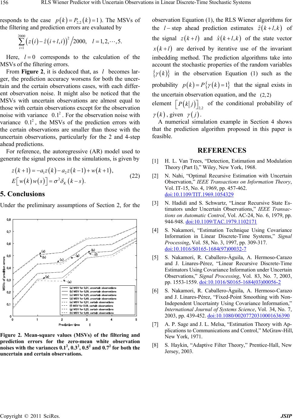

RLS Wiener Predictor with Uncertain Observations in Linear Discrete-Time Stochastic Systems 156
responds
redated by
to the case
 
2,2 1pkP k). The MSVs of
the filtering and p
observation Equation (1), the RLS Wiener algorithms for
the l

step ahead prediction estimates of
the signal

ˆ,
zk lk


zk l

and

ˆ,
iction errors are evalu
 


x
klk of the state vector


x
kl

are derived by iterative use of the invariant
imbedding method. The prediction algorithms take into
account the stochastic properties of the random variables




k  in the observation Equation (1) such as the
probability






1kpk P 

 that the signal exists in
the uncertain observation equation, and the
(2,2)
2000 2
ˆ,2000,1,2, ,5.zizi lil 

1i
Here, corresponds to the calculation f the
MSVs of the filtering errors.
igur
ns for both the uncer-
ta
s
process in the simulations, is give
5. Conclusions
y assumptions of Section 2, for
0lo
From F e 2, it is deduced that, as l becomes lar-
ger, the prediction accuracy worse
in and the certain observations cases, with each differ-
ent observation noise. It might also be noticed that the
MSVs with uncertain observations are almost equal to
those with certain observations except for the observation
noise with variance 2 0.1 . For the observation noise with
variance 2 0.1 , the MSVs of the prediction errors with
the certain observatiare smaller than those with the
uncertain ob ervations, particularly for the 2 and 4-step
ahead predictions.
For reference, the autoregressive (AR) model used to
generate the signal
ons
element


2,2
Pkj



 of the conditional probability of


k  , given


j  .
A numerical simulation example in Section 4 shows
that the prediction algorithm proposed in this paper is
feasible.
REFERENCES
n by
 
12
111,zkazk azkwk (22)
[1] H. L. Van Trees, “Detection, Estimation and Modulation
Theory (Part I),” Wiley, New York, 1968.
[2] N. Nahi, “Optimal Recursive Estimation with Uncertain
Observation,” IEEE Transactions on Information Theory,
Vol. IT-15, No. 4, 1969, pp. 457-462.
doi:10.1109/TIT.1969.1054329
  
2.
K
Ewkwsk s   

[3] N. Hadidi and S. Schwartz, “Linear Recursive State Es-
timators under Uncertain Observations,” IEEE Transac-
tions on Automatic Control, Vol. AC-24, No. 6, 1979, pp.
944-948. doi:10.1109/TAC.1979.1102171
Under the preliminar the
[4] S. Nakamori, “Estimation Technique Using Covariance
Information in Linear Discrete-Time Systems,” Signal
Processing, Vol. 58, No. 3, 1997, pp. 309-317.
doi:10.1016/S0165-1684(97)00032-7
[5] S. Nakamori, R. Caballero-Águila, A. Hermoso-Carazo
and J. Linares-Pérez, “Linear Recursive Discrete-Time
Estimators Using Covariance Information under Uncertain
Observations,” Signal Processing, Vol. 83, No. 7, 2003,
pp. 1553-1559. doi:10.1016/S0165-1684(03)00056-2
[6] S. Nakamori, R. Caballero-Águila, A. Hermoso-Carazo
and J. Linares-Pérez, “Fixed-Point Smoothing with Non-
Independent Uncertainty Using Covariance Information,”
International Journal of Systems Science, Vol. 34, No. 7,
2003, pp. 439-452. doi:10.1080/00207720310001636390
[7] A. P. Sage and J. L. Melsa, “Estimation Theory with Ap-
plications to Communications and Control,” McGraw-Hill,
New York, 1971.
Figure 2. Mean-square values (MSVs) of the filtering and
prediction errors for the zero-mean white observatio n [8] S. Haykin, “Adaptive Filter Theory,” Prentice-Hall, New
Jersey, 2003.
noises with the variances 0.12, 0.32, 0.52 and 0.72 for both the
uncertain and certain observations.

RLS Wiener Predictor with Uncertain Observations in Linear Discrete-Time Stochastic Systems157
et us introduce the equation concerned with the function
Appendix A. Proof of Theorem 1
L

,
J
ks as

,TT JksRspsB sH
 
1
,(
) ,
kT
i
.
J
kiEisHK isH








(A-1)
From (11) and (A-1) it follows that

(A-2)
putting
in (A-1) from (A-1) yields
,

,,, .hk lskAk lJks
Subtracting the equation obtained by
1kk
 


 
,1,
,
JksJksRs

  
 
1
1
,1
,
,.
T
k
i
T
J
kk EksHK 



ksH
Jk
i Jki
EisHKisH






 


 (A-3)
From (A-1), (A-3) and the relationship
, it follows that

2,2
EksPkps  

 

,1,
1,,
Jks Jks

2,2
,
1.
J
kkPkHA
sk


kJk s

 (A-4)
Putting
s
k in (A-1) yields
 
 
 
 
 
  
 
 
1
1
1
1
2,2
1
2,2
(,)
,,
(,),
,,
,,
1, ,1,
.
TT
T
i
TT
T
kT
i
TT T
k
i
TT
JkkRkpkB kH
JkiEikHKikH
pkB kH
JkkEkk HKkkH
JkiEikHKikH
pk Bk HpkJ kk HK kk H
k
J
kiJkkPkHAkJki
piPkHBiA kH




















 




(A-5)
Here, the relationship

 
Ekkpk

  

, (4) and
(A-4) are used. Let us introduce a function
Hence,
 
1
k
i
rk J

 (A-6)
 
,kipiHBi.


 

 

  
 

2,2
1
2
2,2
,
1
,
1.
TT TT
T
T
Jkk
pkBkHrkA kHPk
Rk pkHKkkH
PkHAkrk Ak





(A-7)
Subtracting the equation obtained by putting
in (A-6) from (A-6) yields 1kk





 
    
 
 
  
1
1
1
2,2
1,
,1,
,
,1
,1
k
i
i
rk rkJkkpkHBk
JkiJki piHBi
JkkpkHBk
  
1
2,2 ,
k
.
J
kk piHBi
JkkpkHBkPkHAkrk









Pk HAkJ ki



(A-8)
Here, (A-5) and (A-7) have been used. Clearly, from
(A-6), the initial condition for the recursive Eq
(A-8) of
uation


rk at 0k

is given by
The

00r.
ahiction estiead predmate

l

step

ˆ,
x
klk of


x
kl

is given by (5). From (5) and (Aws -2), it follo
that

1
ˆ,,.
i
k
x
klk AklJkiyi


 (A-9)
Let us uce ation introd func
Hence, the
 
1
,
k
i
ek Jkiyi

. (A-10)
l

step ahead prediction estimate


ˆ,
x
klk of the state vector

x
kl and the filtering
estimate


,
ˆ
x
kk of the state vector

x
k are given by






ˆˆ ,,
 
,
x
klkAklekxkkAkek. (A-11)
Subtracting the equation obtained by
in (A-10) from (A-10) yields
putting
1kk





1
1
.
k
ek
   
1
,, 1,
i
ek
J
kkykJkiJ kiyi






 (A-12)
From (A-4) and (A-10), we get






1,ek Jkkyk
 


1
2,2
1
2,2
,1
,(
k
i
ek
,
1.
J
kk Pk HAkJ kiyi
JkkykPkHAkek






(A-13)
ws that From (A-2), (A-11) and (A-13), it follo

RLS Wiener Predictor with Uncertain Observations in Linear Discrete-Time Stochastic Systems 158
 





2,2
ˆˆ
,1,1
ˆ
,,1,1,
ˆ0,00,
ˆˆ
,1,1
ˆ,0 0.
xkkxk k
hkkkykPkHxkk
x
xk lkxk lk
xl





 

2,2 ˆ
,, 1,1,
lhkkkykPkHxkk 
(A-14)
Introducing
 


,
T
SkAkrkA k
it follows, from (A-8) and (A-15), that
(A-15)








 


2,2
2,2
(1) (,)
1
(1) ,,
,1
00.
T
T
T
T
SkAkrkA kAkJkk
pkHBkPkHAkrkA k
Sk hkkk
pkHKkkPkH Sk
S

 




Finally, the filter gain



,, ,hkkk AkJkk is
expressed as follows








 

2,2
1
2
2,2
,, ,1
(),1 .
TT
TT
hkkkpkKkkHPkSkH
Rkpk HK kk HPk HSk
T




(Q.E.D.)
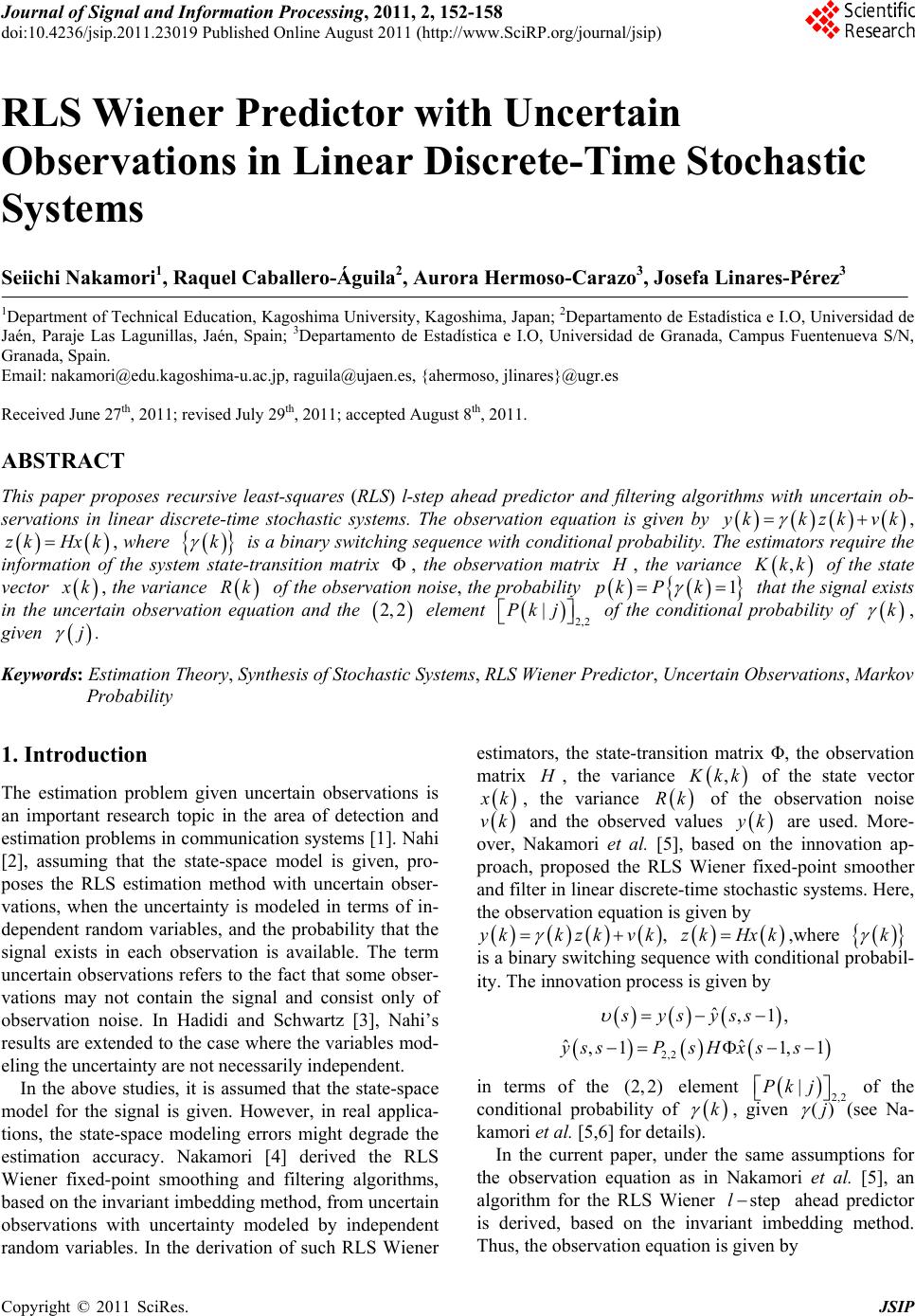