Journal of Signal and Information Processing, 2011, 2, 141-151
doi:10.4236/jsip.2011.23018 Published Online August 2011 (http://www.SciRP.org/journal/jsip)
141
Modeling and Generating Organ Pipes
Self-Sustained Tones by Using ICA
Angelo Ciaramella1, Enza De Lauro2, Salvatore De Martino2, Mariar o sa ri a Fala nga2,
Roberto Tagliaferri3
1Department of Applied Science, University of Naples “Parthenope,” Centro Direzionale, Naples, Italy; 2University of Salerno,
Fisciano, Italy; 3Department of Computer Science, University of Salerno, Fisciano, Italy.
Received June 7th, 2011; revised July 10th, 2011; accepted July 19th, 2011.
ABSTRACT
Aim of this work is to analyze and to synthesize acoustic signals emitted by organ pipes. An Independent Component
Analysis technique is applied to study the behavior of single notes or chords obtained in real and simulated environ-
ments. These analyses suggest that the pipe acoustic signals can be described by a mixture of nonlinear oscillations
obtained by a self-sustained feedback system (i.e., Andronov oscillator). This system allows to obtain a realistic pipe
waveform with features very similar to the sound produced by the pipe and to propose an additive synthesis model.
Moreover, suitable analogical and integrate circuit models, able to reproduce the registered waveforms and sound,
have been designed. A comparison between real and reconstructed acoustic signals is provided.
Keywords: Independent Component Analysis, Sound Synthesis, Non-Linear Oscillators, Integrate Circ uit s
1. Introduction
One of the challenge of the researchers working in music
field is to generate and to control the sound. A synthe-
sizer (or synthesiser) is an electronic instrument able to
reproduce musical sounds. Sound can be produced by
electrical oscillators which are fed to filters (analog syn-
thesizer), or by performing mathematical operations in a
microprocessor (digital synthesizers). Both analog and
digital synthesized sounds may sound dramatically dif-
ferent than recordings of natural sounds. There are also
many different kinds of synthesis methods, each applica-
ble to both analog and digital synthesizers. These tech-
niques tend to be mathematically related, especially the
frequency modulation and the phase modulation. Exam-
ples of these methods are subtractive, frequency modula-
tion, physical modeling, sample based synthesis and so
on [1]. We also note that the sound envelope is used in
many synthesizers, samplers, and other electronic musi-
cal instruments. Its function is to modulate some aspects
of the instrument’s sound. The envelope may be a dis-
crete circuit or module (in the case of analog devices), or
implemented as part of the unit software (in the case of
digital devices). When a mechanical musical instrument
produces sound, the volume of the sound produced
changes over time in a way that varies from instrument to
instrument. The envelope is a way to tailor the timbre for
the synthesizer, sometimes to make it sound more like a
mechanical instrument. For example, a quick attack with
little decay helps it to play more like an organ; a longer
decay and zero sustain makes it more like a guitar. In any
case, any method to synthesize sound is based on a
physical model. The first modeling of the sound produc-
tion and of the acoustics of the musical instruments is the
linear harmonic approximation. This approximation can
be suitable for some instruments such as guitar, piano,
etc., whereas it fails for other instruments such as wind
instruments, whose sound is produced by a nonlinear
mechanism [2,3].
In this paper, we study the organ pipes that are par-
ticular wind instruments in which the nonlinearity does
not depend on the coupling between instrument and
player but it is intrinsic. The now working model of the
organ pipes relies upon the mode-mode coupling and
multiphonic sound production [4]. We investigate the
real acoustic signals emitted by organ pipes with the aim
to reproduce their emitted sound. We propose an additive
synthesis model based on a simple valve analogical cir-
cuit. This model is able to reproduce sounds similar to
the recoded ones both in the waveforms and in the lis-
tening. To reach this goal, we have recorded signals in
several experiments and we have applied well established

Modeling and Generating Organ Pipes Self-Sustained Tones by Using ICA 142
techniques of nonlinear processing operating in the time
domain. A particular role in this analysis is covered by
the Independent Component Analysis (ICA) [5]. It allows
to establish whether the experimental time series are a
linear superposition of statistically independent sources.
The other step is the noise reduction of the decomposed
signals [6]. Indeed, in experimental data, even decom-
posed into simpler sources, a contribution of residual
noise is still relevant.
The de-noised components are the basis for the recon-
struction of the phase space [7-9]. The estimation of the
embedding dimension and of the other extracted infor-
mation allow to recognize the class of dynamical systems
that characterizes the dynamics generating the experi-
mental series [10].
Finally, numerical simulations and comparative simple
methods lead to very simple equations that reproduce
signals even in the listening as confirmed by a formal
AB-preference test [11]. These equations, i.e., a low di-
mension dynamical system, represent on average the
behavior of the complete fluid-dynamical equations de-
scribing the phenomenon. We stress that this model pro-
vides a nonlinear waveform that is highly correlated with
the original pipe sound signal (including the envelope).
In other words, we can reproduce the timbre of the pipe
sound including the attack, decay, sustain and release
phases by using an analogical circuit.
The paper is organized as follows. In Section 2 we in-
sert a brief introduction of the organ pipes. In Section 3
we focus our attention on the description of the wind
instruments remarking their nonlinear features. In Sec-
tion 4 we introduce the ICA approach and the FastICA
algorithm, and in Section 5 a noise reduction method is
described. In Section 6 we present the experiments ob-
tained on real data and we propose the analogical model
to reproduce the registered waveforms. The conclusions
are described in Section 8.
2. Organ Pipe Ranks
The pipe organ is essentially a mechanized wind instru-
ment of the panpipe type. Each pipe is a simple sound
generator optimized to produce just one note with a par-
ticular loudness and timbre, and the organ mechanism
directs air to particular combinations of pipes to produce
the desired soun d. A set of pipes of uniform tone qu ality,
with one pipe for each note over the compass of the or-
gan keyboard, is called rank. The pipes are set out logi-
cally, and generally to a large extent physically, in a ma-
trix. Each row of the matrix contains the pipes of a single
rank and each column of the matrix contains all the pipes
for a single note. There are two types of ranks: flues and
reeds. Flue pipes, also called labial (the upper lip of the
mouth is important in sound production) belong to the
flute-instrument family. Open flue pipes are historically
the basis of the pipe organ and still pro v ide its foundatio n
sound. We can also have stopped flue pipes [3]. In addi-
tion, there are various partly stopped pipes in which the
stopper has a vent or chimney to produce special effects.
Reed pipes, or lingual, have a metal tongue vibrating
against a rather clarinet-like structure called a shallot.
There are two major classes of reeds: those with full
length conical resonators supporting all harmonics and
those half-length cylindrical resonators supporting pri-
marily the odd harmonics. In addition, we find short reed
pipes with cavity resonators rather like trumpet mutes,
but they are quite unusual in modern organs. In virtually
all natural sounds, increase loudness is associated not
simply with a uniform increase in sound pressure level at
all frequencies, but rather with a change in the slope of
the frequency spectrum to give more weight to compo-
nents of higher frequencies. This is a natural cones-
quence of the nonlinearities associated with the produc-
tion of such sounds. We also note that the air column in a
cylindrical pipe is only approximately harmonic in its
resonances [12]. In [3] is demonstrated the mechanism
that provides con siderable nonlinearity for the generation
of the harmonics which are then amplified by the reso-
nator (or not amplified, in the case of even harmonics
and a stopped cylindrical pipe). It also provides the
mechanism for mode locking and, when the conditions
are satisfied, for multiphonic production. The pipe organ
is a very complex instrument, with thousands of pipes at
a multitude of pitches, all under the control of a single
organist.
3. Sustained-Tone Instruments and
Nonlinearity
Musical instruments are often thought as linear harmonic
systems. A closer examination, however, shows that the
reality is very different from this.
Sustained-tone instruments, such as violins, flutes and
trumpets, have resonators that are only approximately
harmonic, and their operation and harmonic sound spec-
trum both rely upon the extreme nonlinearity of their
driving mechanisms. It is helpful to consider the whole
system made of the sustained-tone instrument and its
player, as shown in Figure 1. The instrument itself gen-
erally has a primary harmonic resonator that is main-
tained in oscillation by a power source provided by the
player, together with a secondary resonator, generally
with some broad and inharmonic spectral properties, that
acts as a radiator for the oscillations of the primary reso-
nator. In the linear harmonic approximation, the genera-
tor is assumed simply to provide a negative resistance to
overcome the mechanical and acoustic losses in the pri-
mary resonator, but no information is provided about the

Modeling and Generating Organ Pipes Self-Sustained Tones by Using ICA143
player
steady
energy
source
primary
resonator
negative
resitance
generator
taut string
air column
bow friction,
vibrating reed
vibrating lips
muscles,
breath
Figure 1. System diagram for a sustained-tone musical in-
strument. In most cases the generator is highly nonlinear
and all the other elements are linear.
spectral envelope, and thus about the tone quality of the
sound.
Wind instruments are rather different, in that the pri-
mary resonating body is a air column, which also radiates
the sound. There is th erefore one less element in the total
system diagram. In the more detailed nonlinear treatment,
the generator is usually highly nonlinear, and it is
strongly co upled with the primary resonator. Th e latter is
usually appreciably inharmonic in its modal properties.
The feedback coupling between the resonator and the
generator therefore assumes prime importance in deter-
mining the instrument behavior.
4. The ICA Method
ICA is a method to find underlying factors or compo-
nents from multivariate (multidimensional) statistical
data, based on their statistical independence [5]. In the
simplest form of ICA, one observes m scalar random
variables 12
,,,
m
x
xx which are assumed to be linear
combinations of n unknown independent components
(ICs) denoted b y 12
,,,
n
s
ss. These ICs si are assumed to
be mutually statistically independent, and zero-mean.
Arranging the observed variables xj into a vector
12

T
,
m
,,
x
xxx and the IC variables si into a vector s,
the linear relationship can be expressed as x = As. Here A
is an unknown mxn matrix of full column rank, called the
mixing matrix. The basic problem of ICA is then to esti-
mate both the mixing matrix A and the realizations of the
ICs si using only observations of the mixtures xj. Estima-
tion of ICA requires the use of higher-order statistical
information. Some heuristic approaches have been pro-
posed in literature for achieving separation and some
authors have derived “unsupervised neural” learning al-
gorithms from information-theoretic measures. Among
them, a good measure of independence is given by
negentropy. In the following we shall use the fixed-point
algorithm, namely FastICA, developed to perform linear
mixtures separation by using the negentropy information
[5].
ICA has revealed many interesting applications in dif-
ferent fields of research (bio-medical signals, geophysics,
audio signals, image processing, financial data, etc.). For
instance, it was fruitfully applied in volcanic environ-
ment [8,13], physics of musical instruments [12,14,15]
and dynamical systems in mixtures [16]. Moreover, fur-
ther studies have been conducted on signals recorded in
real environments with delay and reverberation (e.g.,
convolutive mixtures) [17,18].
5. Noise Reduction
The method used in the experiments to accomplish the
nonlinear noise reduction (RNRPCA in the following) is
based on the application of the compression and decom-
pression (reconstruction) of the noise data [6]. To esti-
mate the noise strength we follo wed the heuristic metho d
of Natarajan [19]. Many runs of compression/decom-
pression algorithms of various compression losses, mea-
sured as Peak Signal-to-Noise Ratio (PSNR), have been
tried. After all runs one has to plot the compression ratio
versus PSNR values to obtain the rate-distortion charac-
teristic of the signal. At the point of PSNR corresp onding
to the strength of the noise, the plot of the noisy signal
shows the knee point, that is a point at which the slope of
the curve changes rapidly. The precise determination of
the knee point can be obtained by drawing the second
derivative. The point of PSNR at which the second de-
rivative attains its maximum is the measure of the noise
strength. The practical solution of filtering the random
noise has been obtained through the use of Robust Prin-
cipal Component Analysis Neural Network [14].
6. Experimental Results
The aim of the following experiments is to analyze the
data recorded playing organ pipes, by using the ICA ap-
proach in order to establish how many independent
components, if there are, are necessary to retain all the
information of the recorded signals.
6.1. Recording Data
The first part of our work examines the sound recordings
performed in the church of St. Antonio di Padova located
in Mercato San Severino (SA). We have used a digital
acquisition board with a sampling frequency of 44,100
Hz and nine microphones. The organ is located at three
meters from the principal floor of the church. The mi-
crophones have been positioned linearly along the prin-
cipal floor. Three clusters, composed of three micro-
phones each, have been posed five meters far each other.
In this setup, we have recorded nine signals in each ex-

Modeling and Generating Organ Pipes Self-Sustained Tones by Using ICA 144
periment, recording the notes C, E, G. Furthermore, we
have also performed experiments playing chords. A pre-
liminary analysis of this experimental survey is contained
in [10]. The second part of our work looks at the experi-
ments performed playing an organ pipe in the acoustic
laboratory of Salerno University, where we have used the
same acquisition board and six microphones (see Figure
2 for details of the organ pipes). In these experiments, we
have recorded single notes played with three different
levels of the blowing pressure in order to evidence how
the frequencies depend on the forcing. The pipe blowing
pressure has been supplied by a standard organ mecha-
nism in the church, whereas it is induced by the human
breath at the Department. At the end of the complete
survey, our data set is composed of many scalar series for
each note. The notes are produced by using organ pipe in
different registers and octaves.
6.2. Data Analysis
In the first experiment we focus our attention to analyze
the notes and chords obtained by the organ pipe. The aim
is to analyze this kind of sources, using the FastICA ap-
proach, to study the features of the Dynamical Systems
(D Ss ) t h a t g e n e r a te th e s e s i g n a ls . Ou r data set, taking into
account the linear geometry of the microphones, can be
viewed as different spatial records of the same physical
phenomenon. Before applying FastICA we need to align
the recordings, using cross-correlation, to avoid the de-
lays among the microphones. Analyzing the geometry of
the sampling we conclude that the delay and the rever-
the microphones, the environment and the features of
Figure 2. Organ pipes in the acoustic Laboratory of Salerno
University.
beration in this case can be neglected and then we can
consider a generative model based on instantaneous
mixtures. In our analysis first of all we focus the atten-
tion on the single C note. In Figure 3(a), 9 recorded sig-
nals for the C note and th e relative Power Spectrum Den-
sities (PSDs) are reported. In this case the fundamental
frequency is at 523 Hz. Applying the FastICA approach
to the nine recorded signals we obtain the separation of
three waveforms with the fundamental frequency at 523
Hz and other frequency peaks (see Figure 3(b)). They
are nonlinear signals in limit cycle regime that are line-
arly superimposed. The study of principal components of
the covariance matrix of the signals reveals that there are
only six principal components. Using this information
and applying to these signals the noise reduction method
RNRPCA, we obtain a more clear separation, as we can
see in Figure 3(c). The separated signals are the funda-
mental of the C note with frequency at 523 Hz, one
waveform with lower frequency at 263 Hz and another at
1046 Hz. Moreover, the FastICA approach has extracted
two independent signals more with frequencies of 98 Hz
and 784 Hz. The signal with a main peak eq ual to 98 Hz
can be ascribed the power supply or to G note, whereas
784 Hz signal can be a harmonic of C or another G pipe
in resonance.
In the second experiment, we have considered chords.
In particular, we have played the C, E and G notes si-
multaneously. The estimated sources are related to the
principal modes (C = 523 Hz, E = 331 Hz and G = 393
Hz) and other frequency peaks (C = 262 Hz, E = 663 Hz,
G = 784 Hz and G = 98 Hz). Also in this case we have
applied the RNRPCA algorithm obtaining clearer results.
Coming to the laboratory experiments, we have played
organ pipes under controlled conditions looking at the
sound produced by a single organ pipe without the pres-
ence of the others which could influence the sound. We
have recorded many pipes played with three levels of
blowing pressure: full-toned, intermediate and low level
of pressure. For brevity we report the results relative to
the E note stressing that the acoustic field produced by
the other pipes displays the same features. The record-
ings are preprocessed to avoid the contribution of the
power supply, high-pass filtering the experimental sig-
nals over 50 Hz. To get some knowledge about the dy-
namics generating acoustic signals we have estimated
their phase space and the embedding dimension. The
standard techniques to reconstruct the phase space, based
on the theorem of Takens [9], are well known [7]. To
estimate an upper bound of the attractor dimension, we
used the False Nearest Neighbors (FNN) techniques and
the Average Mutual Information (AMI) [20].
In the experiments illustrated in this paper the embed-
ding dim ensi on of the n ot es i 4. s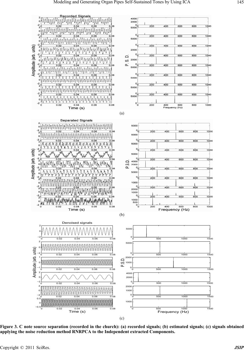

Modeling and Generating Organ Pipes Self-Sustained Tones by Using ICA 145
(a)
(b)
05001000 1500
0
5000
05001000 1500
0
5000
05001000 1500
0
1000
2000
P.S.D.
05001000 1500
0
2000
4000
05001000 1500
0
1000
2000
05001000 1500
0
1000
Frequency (Hz)
00.02 0.04 0.06 0.08
−2
0
2
Denoised signals
00.02 0.04 0.06 0.08
−2
0
2
00.02 0.04 0.06 0.08
−1
0
1
Amplitude (arb. units)
00.02 0.04 0.06 0.08
−2
0
2
00.02 0.04 0.06 0.08
−2
0
2
00.02 0.04 0.06 0.08
−0.5
0
0.5
Time (s)
(c)
Figure 3. C note source separation (recorded in the church): (a) recorded signals; (b) estimated signals; (c) signals obtained
pplying the noise reduction method RNRPCA to the Independent extracted Components. a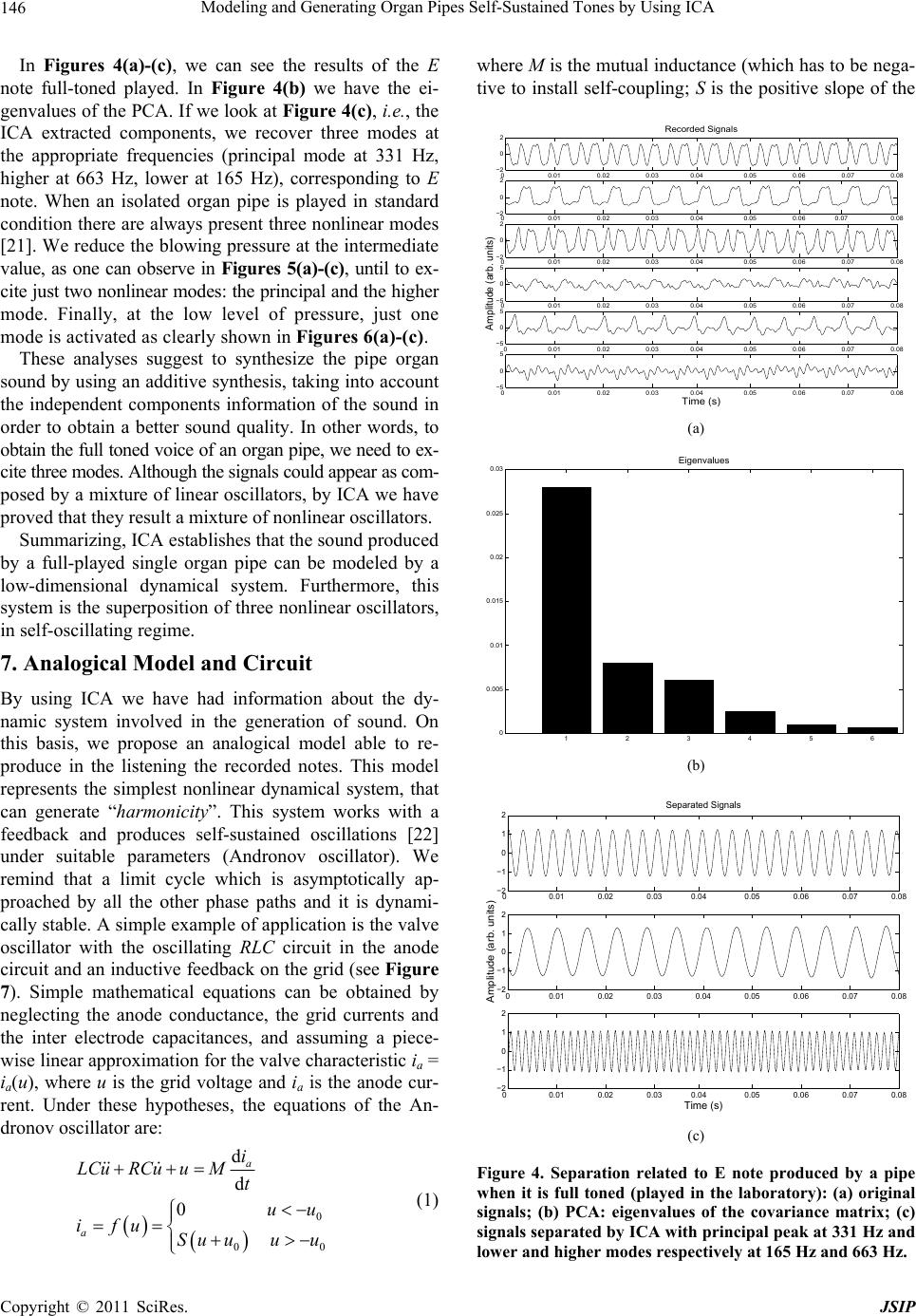

Modeling and Generating Organ Pipes Self-Sustained Tones by Using ICA 146
In Figures 4(a)-(c), we can see the results of the E
note full-toned played. In Figure 4(b) we have the ei-
genvalues of the PCA. If we look at Figure 4(c), i.e., the
ICA extracted components, we recover three modes at
the appropriate frequencies (principal mode at 331 Hz,
higher at 663 Hz, lower at 165 Hz), corresponding to E
note. When an isolated organ pipe is played in standard
condition there are always present three nonlinear modes
[21]. We reduce the blowing pressure at the in termediate
value, as one can observe in Figures 5(a)-(c), until to ex-
cite just two nonlinear modes: the principal and the higher
mode. Finally, at the low level of pressure, just one
mode is activated as clearly shown in Figures 6(a)-( c).
These analyses suggest to synthesize the pipe organ
sound by using an additive syn thesis, taking into account
the independent components information of the sound in
order to obtain a better sound quality. In other words, to
obtain the full ton ed voice of an organ p ipe, we need to ex-
cite three modes. Although the signals could appear as com-
posed by a mixture of linear oscillators, by ICA we have
proved that they result a mixture of nonlinear oscillato rs.
Summarizing, ICA establishes that the sound produced
by a full-played single organ pipe can be modeled by a
low-dimensional dynamical system. Furthermore, this
system is the superposition of three nonlin ear oscillators,
in self-oscillating regime.
7. Analogical Model and Circuit
By using ICA we have had information about the dy-
namic system involved in the generation of sound. On
this basis, we propose an analogical model able to re-
produce in the listening the recorded notes. This model
represents the simplest nonlinear dynamical system, that
can generate “harmonicity”. This system works with a
feedback and produces self-sustained oscillations [22]
under suitable parameters (Andronov oscillator). We
remind that a limit cycle which is asymptotically ap-
proached by all the other phase paths and it is dynami-
cally stable. A simple example of application is the valve
oscillator with the oscillating RLC circuit in the anode
circuit and an inductiv e feedback on the grid (see Figure
7). Simple mathematical equations can be obtained by
neglecting the anode conductance, the grid currents and
the inter electrode capacitances, and assuming a piece-
wise linear approximation for the valve characteristic ia =
ia(u), where u is the grid voltage and ia is the anode cur-
rent. Under these hypotheses, the equations of the An-
dronov oscillator are:


0
00
d
d
0
a
a
i
LCuRCu uMt
uu
ifu Su uuu








 
(1)
where M is the mutual inductance (wh ich has to be nega-
tive to install self-coupling; S is the positive slope of the
0 0.010.020.030.040.050.060.070.08
−2
0
2
Recorded Signals
0 0.010.020.030.040.050.060.070.08
−2
0
2
0 0.010.020.030.040.050.060.070.08
−2
0
2
0 0.010.020.030.040.050.060.070.08
−5
0
5
Amplitude (arb. units)
00.010.020.03 0.040.050.060.070.08
−5
0
5
0 0.010.020.030.040.050.060.070.08
−5
0
5
Time (s)
(a)
123456
0
0.005
0.01
0.015
0.02
0.025
0.03
Eigenvalues
(b)
0 0.010.020.030.040.050.060.070.08
−2
−1
0
1
2
Separated Signals
00.01 0.02 0.03 0.04 0.05 0.06 0.07 0.08
−2
−1
0
1
2
Amplitude (arb. units)
0 0.010.020.030.040.050.060.070.08
−2
−1
0
1
2
Time (s)
(c)
Figure 4. Separation related to E note produced by a pipe
when it is full toned (played in the laboratory): (a) original
signals; (b) PCA: eigenvalues of the covariance matrix; (c)
signals separated by ICA with principal peak at 331 Hz and
lower and higher modes respectively at 165 Hz and 663 Hz.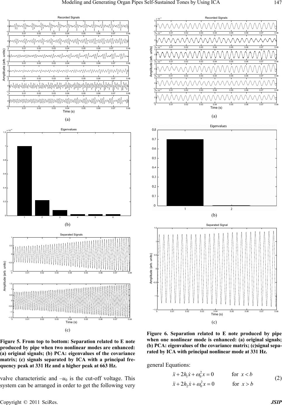

Modeling and Generating Organ Pipes Self-Sustained Tones by Using ICA147
0 0.010.020.030.040.050.060.070.08
−5
0
5
Recorded Signals
0 0.010.020.030.040.050.060.070.08
−5
0
5
0 0.010.020.030.040.050.060.070.08
−5
0
5
0 0.010.020.030.040.050.060.070.08
−5
0
5
Amplitude (arb. units)
00.01 0.02 0.030.040.050.060.07 0.08
−2
0
2
0 0.010.020.030.040.050.060.070.08
−5
0
5
Time (s)
(a)
123456
0
0.2
0.4
0.6
0.8
1
1.2 x 10
−6
Eigenvalues
(b)
0 0.010.020.030.040.050.060.070.08
−1
−0.5
0
0.5
1
Separated Signals
Amplitude (arb. units)
0 0.010.020.030.040.050.060.070.08
−1.5
−1
−0.5
0
0.5
1
1.5
Time (s)
(c)
Figure 5. From top to bottom: Separation related to E note
produced by pipe when two nonlinear modes are enhanc ed:
(a) original signals; (b) PCA: eigenvalues of the covariance
matrix; (c) signals separated by ICA with a principal fre-
quency peak at 331 Hz and a higher peak at 663 Hz.
valve characteristic and –u0 is the cut-off voltage. This
system can be arranged in order to get the following very
0 0.010.020.030.040.050.060.070.08
−5
0
5x 10
−3
Recorded Signals
0 0.010.020.030.040.050.060.070.08
−1
0
1x 10
−3
0 0.010.020.030.040.050.060.070.08
−2
0
2x 10
−3
0 0.01 0.020.030.040.050.060.070.08
−2
0
2x 10
−3
Amplitude (arb. units)
0 0.010.020.030.040.050.060.070.08
−5
0
5x 10
−3
0 0.010.020.030.040.050.060.070.08
−5
0
5x 10
−3
Time (s)
(a)
(b)
0 0.010.020.030.040.050.060.070.08
−1.5
−1
−0.5
0
0.5
1
1.5
Separated Signal
Time (s)
Amplitude (arb. units)
(c)
Figure 6. Separation related to E note produced by pipe
when one nonlinear mode is enhanced: (a) original signals;
(b) PCA: eigenvalues of the covariance matrix; (c)signal sepa-
rated by ICA with principal nonlinear mode at 331 Hz.
general Equations:
2
10
2
20
20 for
20 for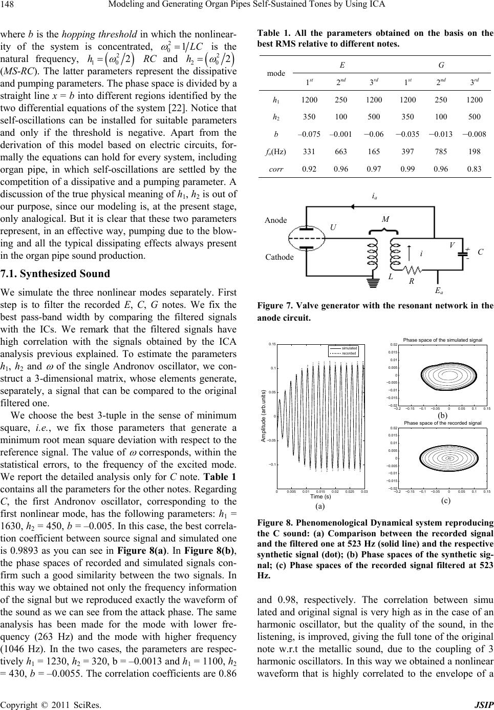
x
hxxx b
x
hxxx b



 

 
 
 
(2)

Modeling and Generating Organ Pipes Self-Sustained Tones by Using ICA 148
where b is the hopping threshold in which the nonlinear-
ity of the system is concentrated, 2
01LC
  is the
natural frequency,

2
10
2h  

RC and


2
20
2h  
(MS-RC). The latter parameters represent the dissipative
and pumping parameters. The phase space is divided by a
straight line x = b into different regions identified by the
two differential equations of the system [22]. Notice that
self-oscillations can be installed for suitable parameters
and only if the threshold is negative. Apart from the
derivation of this model based on electric circuits, for-
mally the equations can hold for every system, including
organ pipe, in which self-oscillations are settled by the
competition of a dissipative and a pumping parameter. A
discussion of the true physical meaning of h1, h2 is out of
our purpose, since our modeling is, at the present stage,
only analogical. But it is clear that these two parameters
represent, in an effective way, pumping due to the blow-
ing and all the typical dissipating effects always present
in the organ pi pe sound production.
7.1. Synthesized Sound
We simulate the three nonlinear modes separately. First
step is to filter the recorded E, C, G notes. We fix the
best pass-band width by comparing the filtered signals
with the ICs. We remark that the filtered signals have
high correlation with the signals obtained by the ICA
analysis previous explained. To estimate the parameters
h1, h2 and  of the single Andronov oscillator, we con-
struct a 3-dimensional matrix, whose elements generate,
separately, a signal that can be compared to the original
filtered one.
We choose the best 3-tuple in the sense of minimum
square, i.e., we fix those parameters that generate a
minimum root mean square deviation with respect to the
reference signal. The value of  corresponds, within the
statistical errors, to the frequency of the excited mode.
We report the detailed analysis only for C note. Table 1
contains all the parameters for the other notes. Regarding
C, the first Andronov oscillator, corresponding to the
first nonlinear mode, has the following parameters: h1 =
1630, h2 = 450, b = –0.005. In this case, the best correla-
tion coefficient between source signal and simulated one
is 0.9893 as you can see in Figure 8(a). In Figure 8(b),
the phase spaces of recorded and simulated signals con-
firm such a good similarity between the two signals. In
this way we obtained not only the frequency information
of the signal but we reproduced exactly the waveform of
the sound as we can see from the attack phase. The same
analysis has been made for the mode with lower fre-
quency (263 Hz) and the mode with higher frequency
(1046 Hz). In the two cases, the parameters are respec-
tively h1 = 1230, h2 = 320, b = –0 .0013 and h1 = 1100, h2
= 430, b = –0.0055. The correlation coefficients are 0.86
Table 1. All the parameters obtained on the basis on the
best RMS relative to different notes.
E G
mode 1st 2nd 3rd 1st 2nd 3rd
h1 1200250 1200 1200 250 1200
h2 350 100 500 350 100 500
b –0.075 –0.001–0.06 –0.035 –0.013 –0.008
fo(Hz) 331 663 165 397 785 198
corr 0.92 0.96 0.97 0.99 0.96 0.83
Ano de
Cathode
Ea
ia
i C
M
U
R
L
V
Figure 7. Valve generator with the resonant network in the
anode circuit.
−0.2 −0.15 −0.1 −0.0500.050.10.1
5
−0.02
−0.015
−0.01
−0.005
0
0.005
0.01
0.015
0.02
Phase space of the simulated signal
00.005 0.01 0.015 0.02 0.025 0.03
−0.1
−0.05
0
0.05
0.1
0.15
Time (s)
Amplitude (arb.units)
−0.2 −0.15 −0.1 −0.0500.050.10.1
5
−0.02
−0.015
−0.01
−0.005
0
0.005
0.01
0.015
0.02
Phase space of the recorded signal
a )b )
c)
simulated
recorded
(a) (c)
(b)
Figure 8. Phenomenological Dynamical system reproducing
the C sound: (a) Comparison between the recorded signal
and the filtered one at 523 Hz (solid line) and the respective
synthetic signal (dot); (b) Phase spaces of the synthetic sig-
nal; (c) Phase spaces of the recorded signal filtered at 523
Hz.
and 0.98, respectively. The correlation between simu
lated and original signal is very high as in the case of an
harmonic oscillator, but the quality of the sound, in the
listening, is improved, giving the full tone of the original
note w.r.t the metallic sound, due to the coupling of 3
harmonic oscillators. In this way we obtained a nonlinear
waveform that is highly correlated to the envelope of a

Modeling and Generating Organ Pipes Self-Sustained Tones by Using ICA149
pipe sound. The main idea, now, is to use these features
to analogical reproduce the real timbre of the pip e sound.
By comparing the synthesized waveform with that ob-
tained from a simple additive synthesis we obtain a more
realistic waveform and sound.
7.2. AB-Preference Test
To validate the introduced nonlinear model we perform a
formal AB-preference test [11] versus the linear oscilla-
tor based model and the recorded notes. In these tests we
select 10 listeners and they are subjected to several notes
processed by the two systems in randomized order. For
each note the listeners have made a preference decision.
In details, in Table 2 the listeners are invited to make
a choice between the modes simulated by using the linear
and nonlinear oscillators. Totally, we have 7 notes simu-
lated by the two models. Each note has been simulated
by the two models varying the number of modes from 1
to 3. We see from these results that a nonlinear model is
preferred in all the cases with higher order percentages.
In Table 3 and Table 4, instead, we have proposed to
make a choice between signals obtained by the nonlinear
model considering the superposition of one and two or
two and three modes, respectively. As confirmed by the
ICA analysis we have that the best performance is asso-
ciated with the modes simulated by using three nonlinear
systems linearly superimposed. Finally, in Table 5 we
detail the results obtained subjecting the listeners to
make a preference between real recorded notes and that
Table 2. AB-preference test between the linear and non-
linear oscillators based models.
Mixture 1 mode 2 modes 3 modes
Linear 23% 14% 7%
Non-Linear 77% 86% 93
Table 3. AB-preference test of the nonlinear oscillator vary-
ing the number of modes: comparison by using 1 and 2
modes.
Model Non-linear
1 mode 31%
2 modes 69%
Table 4. AB-preference test of the nonlinear oscillator vary-
ing the number of modes: comparison by using 2 and 3
modes.
Model Non-Linear
2 modes 29%
3 modes 71%
Table 5. AB-preference test between recording notes and
that simulated by the non-linear oscillator with three modes.
Comparison
recorded 56%
simulated 44%
simulated by the nonlinear oscillator with three modes. In
this case the results show that the proposed model is a
good candidate to appropriately reproduce an organ pipe
waveform note.
7.3. Hardware Schematization
The proposed model permits to obtain a realistic pipe
waveform with features very similar to the source pipe
(included the attack phase). In other words, it is possible
to give an hardware schematization, i.e., design a suitable
integrate circuit, observing that the circuit in Figure 7
can be developed in terms of logical functions adopting
the scheme of Figure 9 by using the MatlabR Simulink.
From the given scheme we see that the main operations
are addition (and substraction) and integration. These
operations could be obtained by using an operational
amplifier. An operational amplifier is a voltage and cur-
rent amplifier obtained by using transistors. The circuit
based on transistors could be more compact than the
valve based one bu t it is knows that the va lve could give
a better fidelity.
8. Conclusions
In this paper we have analyzed acoustic signals emitted
by organ pipes. At a first elementary approximation the
generative model of sound in musical instruments seems
to be linear. But the analysis and models so produced
appear suitable only until the physical processes are in-
vestigated in a little more detail. Indeed, the whole sys-
tem that constitutes a musical instrument is nonlinear.
By using ICA, relevant features of single tones have
been extracted from real data (three nonlinear modes).
This analysis suggests to use an additive model to syn-
thesize the pipe sounds. The decomposition of the notes
and of the chords into independent components provides
sufficient information to model the waveform envelope
together with the transient attack. This permits to have a
better quality sound than that obtained by using simple
additive methods based on linear harmonic oscillators or
that obtained by using spectral analysis of the sound.
We have introduced a simple and suitable analogical
model, able to reproduce the registered waveform and
sound in listening. The mod el provides simulated signals
highly correlated with the original one. Furthermore, the
quality of the sound, in the listening, is improved, giving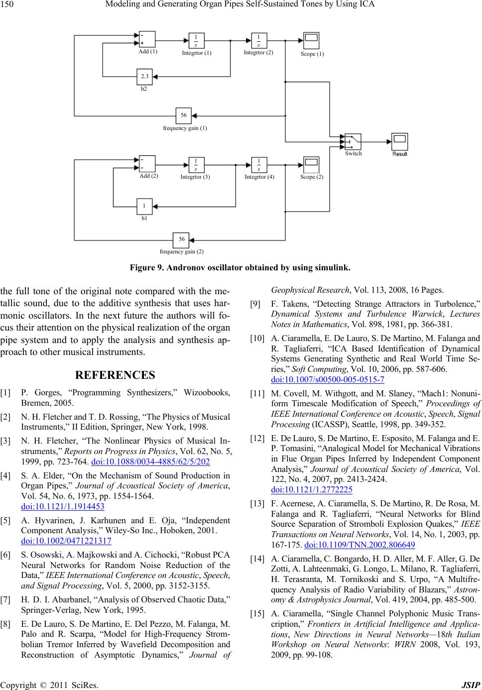

Modeling and Generating Organ Pipes Self-Sustained Tones by Using ICA 150
Integrtor (1)Integrtor (2)
Integrtor (3)Integrtor (4)
Add (1)
Add (2)
Scope (1)
Scope (2)
h2
h1
frequency gain (1)
Switch
frequency gain (2)
2.3
1
56
1
s
1
s
1
s
1
s
56
Figure 9. Andronov oscillator obtained by using simulink.
the full tone of the original note compared with the me-
tallic sound, due to the additive synthesis that uses har-
monic oscillators. In the next future the authors will fo-
cus their attention on the physical realization of the organ
pipe system and to apply the analysis and synthesis ap-
proach to other musical instruments.
REFERENCES
[1] P. Gorges, “Programming Synthesizers,” Wizoobooks,
Bremen, 2005.
[2] N. H. Fletcher an d T. D. Rossing, “The Ph ysics of Musical
Instruments,” II Edition, Springer, New York, 1998.
[3] N. H. Fletcher, “The Nonlinear Physics of Musical In-
struments,” Reports on Progress in Physics, Vol. 62, No. 5,
1999, pp. 723-764. doi:10.1088/0034-4885/62/5/202
[4] S. A. Elder, “On the Mechanism of Sound Production in
Organ Pipes,” Journal of Acoustical Society of America,
Vol. 54, No. 6, 1973, pp. 1554-1564.
doi:10.1121/1.1914453
[5] A. Hyvarinen, J. Karhunen and E. Oja, “Independent
Component Analysis,” Wiley-So Inc., Hoboken, 2001.
doi:10.1002/0471221317
[6] S. Osowski, A. Majkowski an d A. Cichocki, “R obust PCA
Neural Networks for Random Noise Reduction of the
Data,” IEEE International Conference on Acoustic, Speech,
and Signal Processing, Vol. 5, 2000, pp. 3152-3155.
[7] H. D. I. Abarbanel, “Analysis of Observed Chaotic Data,”
Springer-Verlag, New York, 1995.
[8] E. De Lauro, S. De Martino, E. Del Pezzo, M. Falanga, M.
Palo and R. Scarpa, “Model for High-Frequency Strom-
bolian Tremor Inferred by Wavefield Decomposition and
Reconstruction of Asymptotic Dynamics,” Journal of
Geophysical Research, Vol. 113, 2008, 16 Pages.
[9] F. Takens, “Detecting Strange Attractors in Turbolence,”
Dynamical Systems and Turbulence Warwick, Lectures
Notes in Mathematics, Vol. 898, 1981, pp. 366-381.
[10] A. Ciaramella, E. De Lauro, S. De Martino, M. Falanga and
R. Tagliaferri, “ICA Based Identification of Dynamical
Systems Generating Synthetic and Real World Time Se-
ries,” Soft Computing, Vol. 10, 2006, pp. 587-606.
doi:10.1007/s00500-005- 0515-7
[11] M. Covell, M. Withgott, and M. Slaney, “Mach1: Nonuni-
form Timescale Modification of Speech,” Proceedings of
IEEE International Conference on Acoustic, Speech, Signal
Processing (ICASSP), Seattle, 1998, pp. 349-352.
[12] E. De Lauro, S. De Martino, E. Esposito, M. Falanga and E.
P. Tomasini, “Analogical Model for Mechanical Vibrations
in Flue Organ Pipes Inferred by Independent Component
Analysis,” Journal of Acoustical Society of America, Vol.
122, No. 4, 2007, pp. 2413-2424.
doi:10.1121/1.2772225
[13] F. Acernese, A. Cia ra mella , S. De Ma rtino, R. De Rosa, M.
Falanga and R. Tagliaferri, “Neural Networks for Blind
Source Separation of Stromboli Explosion Quakes,” IEEE
Transactions on Neural Networks, Vol. 14, No. 1, 2003, pp.
167-175. doi:10.1109/T NN.200 2.8066 49
[14] A. Ciaramella, C. Bongardo, H. D. Aller, M. F. Aller, G. De
Zotti, A. Lahteenmaki, G. Longo, L. Milano, R. Tagliaferri,
H. Terasranta, M. Tornikoski and S. Urpo, “A Multifre-
quency Analysis of Radio Variability of Blazars,” Astron-
omy & Astrophysics Journal, Vol. 419, 2004, pp. 485-500.
[15] A. Ciaramella, “Single Channel Polyphonic Music Trans-
cription,” Frontiers in Artificial Intelligence and Applica-
tions, New Directions in Neural Networks—18th Italian
Workshop on Neural Networks: WIRN 2008, Vol. 193,
2009, pp. 99-108.

Modeling and Generating Organ Pipes Self-Sustained Tones by Using ICA151
[16] E. De Lauro, S. De Martino, M. Falanga, A. Ciaramella and
R. Tagliaferri, “Complexity of Time Series Associated to
Dynamical Systems In ferred fro m Independent Comp onent
Analysis,” Physical Review E, Vol. 72, 2005, pp. 1-14.
[17] A. Ciaramella, M. Funaro and R. Tagliaferri, “Separation of
Convolved Mixtures in Frequency Domain ICA,” Interna -
tional Journal of Contemporary Mathematical Sciences,
Vol. 1, No. 16, 2006, pp. 769-795.
[18] A. Ciaramella and R. Tagliaferri, “Amplitude and Permuta-
tion Indeterminacies in Frequency Domain Convolved
ICA,” Proceedings of the IEEE International Joint Con-
ference on Neural Networks 2003, Vol. 1, 2003, pp. 708-
713.
[19] B. Natarajan, “Filtering Random Noise from Deterministic
Signals via Data Compression,” IEEE Transactions on
Signal Processing, Vol. 43, 1995, pp. 2595-2605.
doi:10.1109/78.482110
[20] P. Grassberger and I. Procaccia, “Measuring the Strangeness
of Strange Attractors,” Physica D: Nonlinear Phenomena,
Vol. 9, No. 1-2, 1983, pp. 189-208.
[21] L. D. Landau and E. M. Lifshitz, “Fluid Mechanics,” Per-
gamon Press, Oxford, 1959.
[22] A. A. Andronov, A. A. Vitt and S. E. Khaikin, “Theory of
Oscillators,” Republished Dover Publications, Inc., 1966.