Journal of Mathematical Finance, 2011, 1, 34-39
doi:10.4236/jmf.2011.12005 Published Online August 2011 (http://www.SciRP.org/journal/jmf)
A Comparison of Minimum Risk Portfolios under the
Credit Crunch Crisis
Theodoros Mavralexakis1, Konstantinos Kiriakopoulos2,3, George Kaimakamis4, Alexandros Koulis3
1Proton Bank, Risk Management Department, Athens, Greece
2Proton Bank, Capital Markets, Athens, Greece
3Department of Regional Economic Development, University of Central Greece, Lamia, Greece
4Department of Mathematics and Applied Mechanics, Hellenic Army Academy, Athens, Greece
Received July 4, 2011; revised July 24, 2011; accepted August 2, 2011
Abstract
In this paper the behaviour of various popular risk portfolios measures used for portfolio construction are
compared using data from the recent financial crisis. Results are revealing the way optimal portfolios should
be constructed. Despite the conventional wisdom, short selling gives only a marginal improvement to portfo-
lio performance during the crisis period. Optimal semivariance portfolio produces better results than the
portfolio constructed with the more advanced expected short fall method. Additional historical information
has added to performance up to a point and long dated history seems not to be commensurate with additional
benefits. Rebalancing frequency seems to have an optimal point that favours neither overtrading nor the
conventional buy and hold strategy.
Keywords: Portfolio Optimization, Expected Shortfall, Minimum Variance
1. Introduction
The financial market turmoil, which emerged in late
2007, has led to the most severe financial crisis since the
Great Depression. The bursting of the housing bubble
forced banks to write off several hundred billion dollars
in bad loans caused by mortgage delinquencies. At the
same time, the stock market capitalization of the major
banks declined by more than twice as much. While the
overall mortgage losses were large on an absolute scale,
they were still relatively modest compared to the $8 tril-
lion of US stock market wealth losses between Oc- tober
2007 when the stock market had reached an all- time
high and October 2008. Stulz [1] mentions the need for
taking into account events of small probability that can
lead to such big losses.
This highlights once again the importance of con-
structing minimum risk portfolios with no implicit nor-
mality assumptions on returns. This work attempts to
search for a methodology to construct optimal minimum
risk portfolios by capitalizing on different risk measures.
Various minimum risk portfolio selection measures, us-
ing data from the recent financial crisis, are compared.
These measures are used ex-ante, and optimal portfolios
are constructed. In this way, the preferences of a risk-
avert investor who wants to choose portfolios ex-ante
based on different minimum risk measures are reflected.
The risk measures optimized are variance (variance
minimization-VM), the Expected Shortfall (ES) and the
semivariance method (SEMI). Results are compared to
the results produced by the naive method (NM) and by
using various benchmark indices. Although the variance
measure ([2]) is criticized for its simplicity since it uses
only the first two moments for portfolio selection and
implicitly assumes normality of portfolio returns, it re-
mains a well-accepted measure at least for comparison
reasons. Modern VAR or ES can be either as a constraint
embedded on broader stochastic portfolio maximization
problem ([3,4]) or as an objective function to be mini-
mized ([3,5-7]).
Extensions when the exit time is uncertain can be
found in [8]. The lack of subadditiv ity of the VAR meas-
ure ([9-11]) makes the ES measure a better candidate for
optimization since it is consistent to risk management
objectives for capital allocation, especially within the
scope of the Basel II regulation framework. VAR/ES
methods has also been extensively used for derivatives
portfolio ([12,13]). Gilli and Schummann [14] investi-

T. MAVRALEXAKIS ET AL. 35
gate the empirical performance of alternative selection
criteria in portfolio optimization. Although the results
presented there have a great sensitivity to small data
perturbations, alternative selection criteria such as the
semivariance measure seems to produce superior results
to the variance measure. This is the reason semivariance
minimization is included in the portfolio selection crite-
ria. The naive method, although has a questionable effi-
ciency ([15]), is used for reasons of comparison since its
diversification is guaranteed. This paper is organized as
follows: In Section 2 the optimization methodology is
presented. Section 3 includes the data used and the soft-
ware employed. Our main results can be found in Section
4. Conclusions and extensions can be found in Section 5.
2. Optimization Methodology
We employ three minimization programs: the variance
minimization, the expected short fall minimization and
the semivariance minimization. The objective is to find
the optimal portfolios that minimize the programs above
and to actually test them during the recent crisis. We use
the following notation:
N: is the number of portfolio assets.
1
T, 2 T: are the first and the last day respectively in the
period under examination.
T: is the number of trading days in the periods [1 T,
2
T].
t: is the first day of portfolio rebalancing.
H: is the number of trading days in the historical win-
dows used for the calculation of portfolio variance,
semivariance or expected shortfall, when needed. It must
hold 1
tT H .
F
: is the number of days until rebalancing. Rebal-
ancing takes place at dates tjF

, 0,, t jL, where
t
L is the integer part of the ratio 2
Tt
F
.

12
,,, T
jjj J
N
  , 0,, t
jL

 represent vector
of the weights in the N assets at the j rebalancing period.
In case of short sale restrictions it holds 01
j
i


.
Moreover, 11
Nj
ii


. Let χ be the set of all possible
admissible portfolio vectors.
Let

12
,,, T
ii i
iN
PPP P be the asset price vector at
the i date. We have the usual budget constraint T
tt
P 

u where 0u. The minimum variance program is the
usual convex minimization program that is perf ormed on
the rebalancing periods:
min
J
T
J
J
V




The variance covariance matrix V is calculated using
daily data from the historical window prior to the rebal-
ancing date.
Following Uryasev et al. (200 2), for the VAR and ex-
pected shortfall program with probability


0,1   we
first define the function ()g

for a portfolio vector






1
1
() ,
1
H
k
k
gfya
H

 



  


where




 is the β-quantile of the portfolio loss
distribution and


,
f
y  is the negative daily portfolio
return with portfolio vector x and portfolio daily re-
turns

1,, T
N
yy y. So we have

,
f
yy




and




() min,aaRP


  where P(χ) is the
probability of


,
f
y  not exceeding the α threshold.
The daily portfolio returns are calculated from the port-
folio vector prices as a log returns.
The VAR and expected shortfall program is

min
j
j
g



where the optimization is performed on the rebalancing
periods 0,, t jL

. This setting of minimizing


j
g

is a problem of convex programming as

j
g

is con-
vex as a function of x and VAR and therefore differenti-
able in these variables. If ˆ
j

is the optimal portfolio
vector at the rebalancing date j then the VAR is


ˆ
j
a


and the expected shortfall is

ˆ
j
g

.
Finally the semivariance optimization program is ob-
tained similarly to the minimum variance optimization
but now instead of variance of returns, the partial mo-
ment of semivariance ([16]) is used. It is clear from the
above that on each rebalancing date three optimization
programs are performed and the optimal VM portfolio,
the min imu m V AR /E S po rtf ol io and th e mi ni mum S EM I
portfolio are obtained.
3. Data and Software
Four different data sets with only risky assets were con-
sidered and time series of closing prices spanning from
1/11/1997 to 3/3/2009 were used. The credit crunch pe-
riod was from 1/11/2007 to 3/3/2009 . The data sets were
composed of big capitalization stocks, listed in the Greek,
European and US market and two zero Greek govern-
ment coupon bonds with maturities of two and ten years.
Greek market has been chosen, because it is within the
euro area but still has emerging markets characteristics
like increased volatility, increased bid-offer spreads and
lack of depth compared to the core European markets
during periods of crises. Also the Greek bond market is
very suitable for this analysis because on the one hand it
is very liquid and is quoted on a spread to the German
bond market and on the other hand during the recent cri-
sis has been more damaged compared to other European
or American markets. Since in the analysis only risky

T. MAVRALEXAKIS ET AL. 36
assets are considered, Greek bonds used present a risky
class albeit of different nature from stocks. The bond
maturities used were capturing the most part of the yield
curve, and zero coupon were chosen so that the rein-
vestment coupon problem to be avoided.
Stocks with sufficient data history, which cover at
minimum the historical window, were grouped by their
national market and formed different data sets. The data
sets are the following: 1) 24 different time series of
stocks included in FTSE20 and FTSE40 Greek indexes;
2) 24 time series of stocks included in Dax30 Index; 3)
29 time series of stocks included in Dow 30 index and 4)
time series of ASE, Dax 30, Dow 30 indexes plus time
series of 10 years and 2 years Greek zero coupon bonds.
The formation of the objective function was based on
historical distribution and risk measures instead of risk
reward ratios (i.e. sharp ratios) were optimized. Keeping
the number of assumption to the minimum, rebalancing
frequencies, historical windows, risk measures, data
groups and short sales indicators were all variables to be
optimized during the credit crunch period.
During the credit crunch period rolling- window back-
-tests with a historical window of length H, and a holding
period of length F, were conducted. Overall, the time
evolution of 1440 different portfolios by using 4 histori-
cal windows, 9 rebalancing periods, 5 risk measures, 4
data groups and 2 short sales on/off indicators were
tested.
Each one of the different historical windows consid-
ered was of length 1 year, 2 years, 5 years and 10 years
and each one of the hold ing periods was of length 1 day,
1 week, 2 weeks, 1 month, 2 months, 3 months, 4 months,
5 months and 8 months.
Thus, at point in time 1 t, on data from 1 tH

to
11t, optimization is performed with the resulting port-
folio to be held until 21
ttF . At this point, a new
optimal portfolio is computed, using data from 2
tH

until 21t, and the existing portfolio is rebalanced. This
new portfolio is then held until 32 ttF and so on
and so forth until the end of the period. So during the
walk forward through the data, wealth trajectories are
computed optimizing each one of the above variables
considered and holding the others fixed. In order to per-
form the wealth trajectories through time, the initial port-
folio was set to contain only cash in amount of 100,000
EUR. No limits were imposed on the individual positions
i

. The optimal values for each of the above variables,
formed the selection criteria of the optimal portfolio to
be tested against indexing and equal weight strategies.
The software used for the computations was Matlab
R2007b. Optimizations were performed using sequential
quadratic programming methods (SQP), which transform
the constrained optimization problem into an easier sub-
problem that can then be solved and used as the basis of
an iterative process. Fmincon function capitalizes on this
method by solving the constrained problem using a se-
quence of parameterized quadratic programming uncon-
strained optimizations (more details about fmincon and
constraint non linear optimization exist in http://www.
mathworks.com).
4. Results
4.1. Risk Measures Performance
Interesting results were drawn concerning the choice of
the optimal risk measure, the optimal rebalancing period,
the optimal historical window and the usage or not of
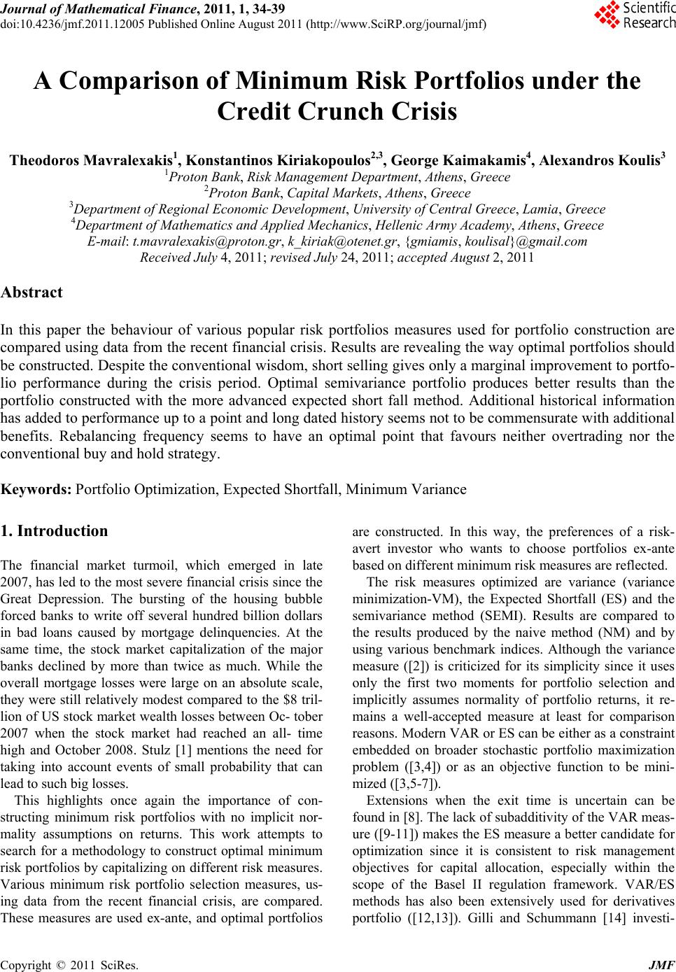
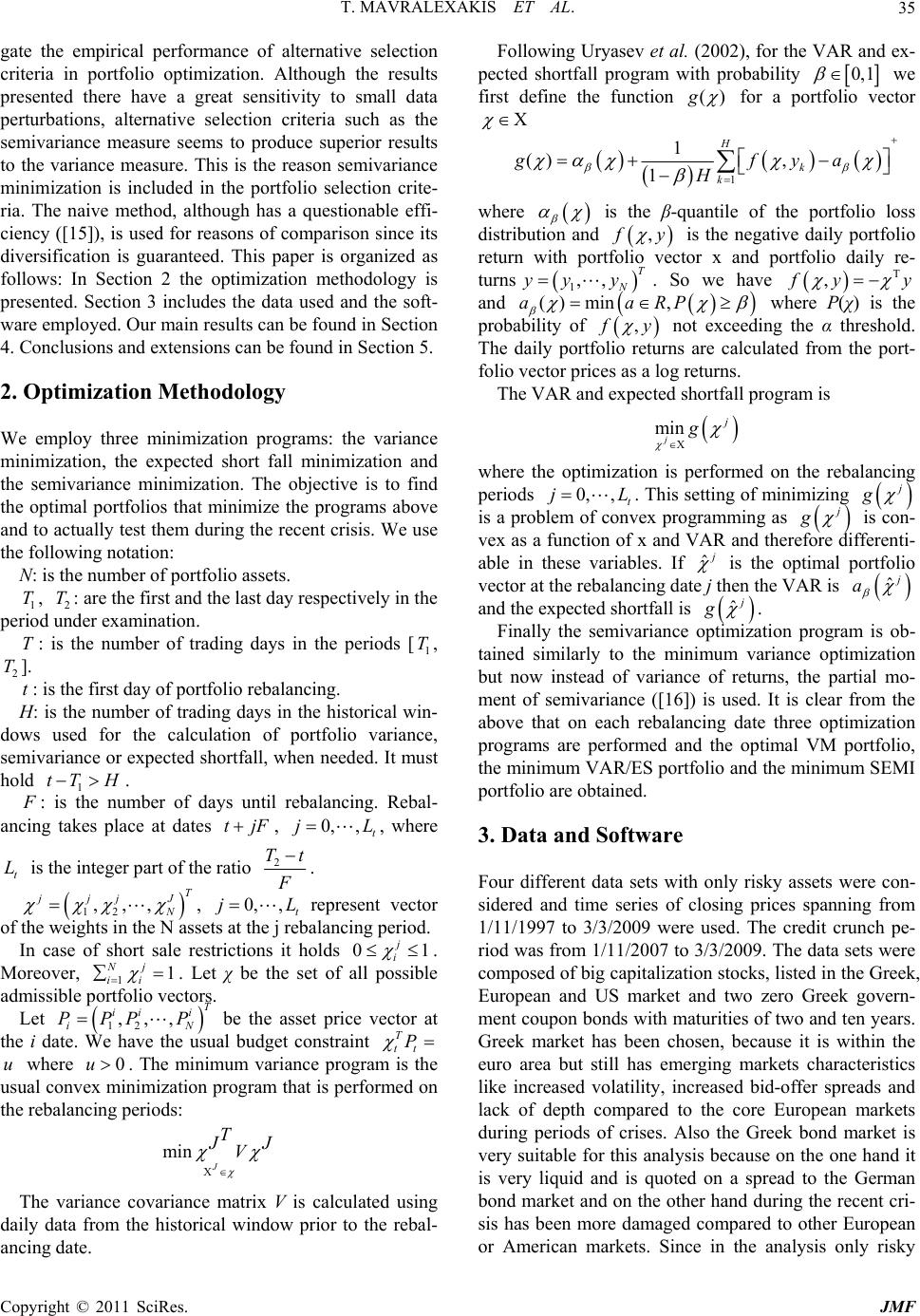
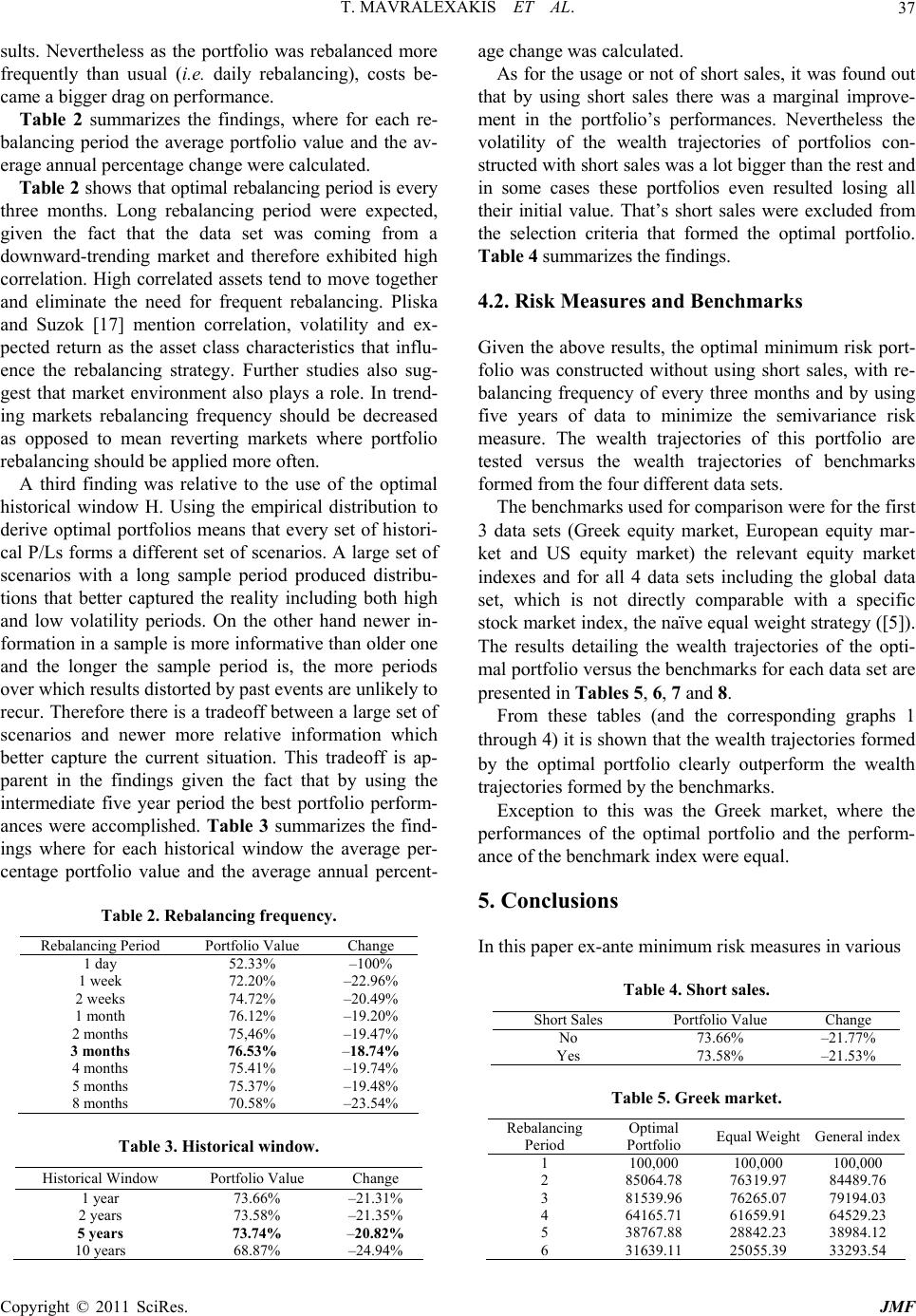
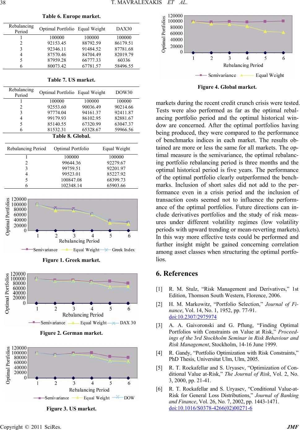
short sales. The main result from the comparison of the
risk measures was that portfolios constructed by mini-
mizing partial and conditional moments like SEMI and
ES performed better than those constructed by simply
minimizing variance. Furthermore, when considered con-
fidence levels for the ES methodology, the optimal level
was the 95% and not 90% or 99% confidence levels.
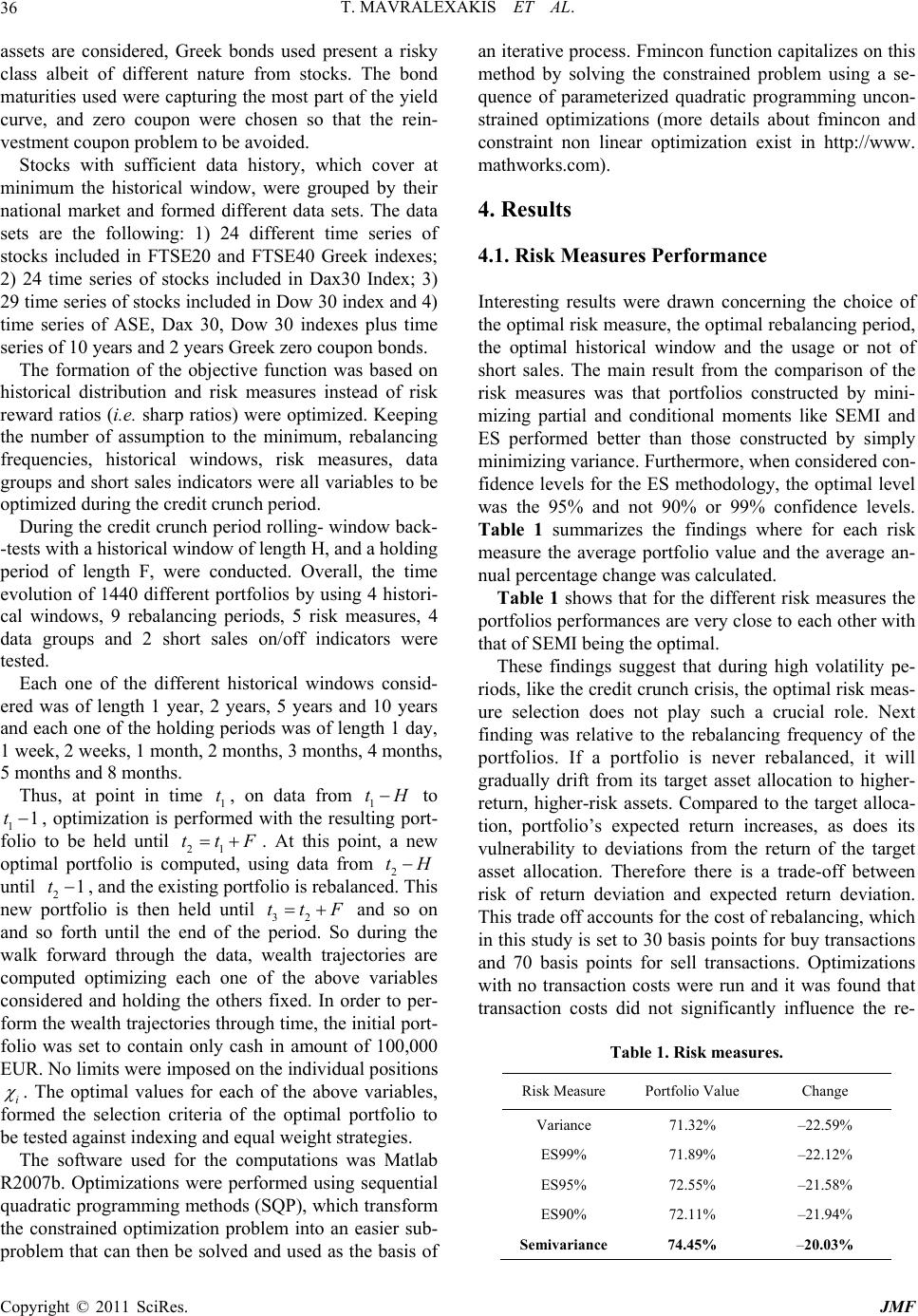
Table 1 summarizes the findings where for each risk
measure the average portfolio value and the average an-
nual percentage change was calculated.
Table 1 shows that for the different risk measures the
portfolios performances are very close to each other with
that of SEMI being the optimal.
These findings suggest that during high volatility pe-
riods, like the credit crunch crisis, the optimal risk meas-
ure selection does not play such a crucial role. Next
finding was relative to the rebalancing frequency of the
portfolios. If a portfolio is never rebalanced, it will
gradually drift from its target asset allocation to higher-
return, higher-risk assets. Compared to the target alloca-
tion, portfolio’s expected return increases, as does its
vulnerability to deviations from the return of the target
asset allocation. Therefore there is a trade-off between
risk of return deviation and expected return deviation.
This trade off accounts for the cost of rebalancing, which
in this study is set to 30 basis points for buy transactions
and 70 basis points for sell transactions. Optimizations
with no transaction costs were run and it was found that
transaction costs did not significantly influence the re-
Table 1. Risk measures.
Risk Measure Portfolio Value Change
Variance 71.32% –22.59%
ES99% 71.89% –22.12%
ES95% 72.55% –21.58%
ES90% 72.11% –21.94%
Semivariance 74.45% –20.03%

T. MAVRALEXAKIS ET AL. 37
sults. Nevertheless as the portfolio was rebalanced more
frequently than usual (i.e. daily rebalancing), costs be-
came a bigger drag on performance.
Table 2 summarizes the findings, where for each re-
balancing period the average portfolio value and the av-
erage annual percentage change were calculated.
Table 2 shows that optimal rebalancing period is every
three months. Long rebalancing period were expected,
given the fact that the data set was coming from a
downward-trending market and therefore exhibited high
correlation. High correlated assets tend to move together
and eliminate the need for frequent rebalancing. Pliska
and Suzok [17] mention correlation, volatility and ex-
pected return as the asset class characteristics that influ-
ence the rebalancing strategy. Further studies also sug-
gest that market environment also plays a role. In trend-
ing markets rebalancing frequency should be decreased
as opposed to mean reverting markets where portfolio
rebalancing should be applied more often.
A third finding was relative to the use of the optimal
historical window H. Using the empirical distribution to
derive optimal portfolios means that every set of histori-
cal P/Ls forms a different set of scenarios. A large set of
scenarios with a long sample period produced distribu-
tions that better captured the reality including both high
and low volatility periods. On the other hand newer in-
formation in a sample is more informative than older one
and the longer the sample period is, the more periods
over which results distorted by past events are unlikely to
recur. Therefore there is a tradeoff between a large set of
scenarios and newer more relative information which
better capture the current situation. This tradeoff is ap-
parent in the findings given the fact that by using the
intermediate five year period the best portfolio perform-
ances were accomplished. Table 3 summarizes the find-
ings where for each historical window the average per-
centage portfolio value and the average annual percent-
Table 2. Rebalancing frequency.
Rebalancing Period Portfolio Value Change
1 day 52.33% –100%
1 week 72.20% –22.96%
2 weeks 74.72% –20.49%
1 month 76.12% –19.20%
2 months 75,46% –19.47%
3 months 76.53% –18.74%
4 months 75.41% –19.74%
5 months 75.37% –19.48%
8 months 70.58% –23.54%
Table 3. Historical window.
Historical Window Portfolio Value Change
1 year 73.66% –21.31%
2 years 7 3.58% –21.35%
5 years 73.74% –20.82%
10 years 68.87% –24.94%
age change was calculated.
As for the usage or not of short sales, it was found out
that by using short sales there was a marginal improve-
ment in the portfolio’s performances. Nevertheless the
volatility of the wealth trajectories of portfolios con-
structed with short sales was a lot bigger than the rest and
in some cases these portfolios even resulted losing all
their initial value. That’s short sales were excluded from
the selection criteria that formed the optimal portfolio.
Table 4 summarizes the findings.
4.2. Risk Measures and Benchmarks
Given the above results, the optimal minimum risk port-
folio was constructed without using short sales, with re-
balancing frequency of every three months and by using
five years of data to minimize the semivariance risk
measure. The wealth trajectories of this portfolio are
tested versus the wealth trajectories of benchmarks
formed from the four different data sets.
The benchmarks used for comparison were for the first
3 data sets (Greek equity market, European equity mar-
ket and US equity market) the relevant equity market
indexes and for all 4 data sets including the global data
set, which is not directly comparable with a specific
stock market index, the naïve equal weight strategy ([5]).
The results detailing the wealth trajectories of the opti-
mal portfolio versus the benchmarks for each data set are
presented in Tables 5, 6, 7 and 8.
From these tables (and the corresponding graphs 1
through 4) it is shown that the wealth trajectories formed
by the optimal portfolio clearly outperform the wealth
trajectories formed by the benchmarks.
Exception to this was the Greek market, where the
performances of the optimal portfolio and the perform-
ance of the benchm ark index were equal.
5. Conclusions
In this paper ex-ante minimum risk measures in various
Table 4. Short sales.
Short Sales Portfolio Value Change
No 73.66% –21.77%
Yes 73.58% –21.53%
Table 5. Greek market.
Rebalancing
Period Optimal Portfolio Equal Weight General index
1 100,000 100,000 100,000
2 85064.78 76319.97 84489.76
3 81539.96 76265.07 79194.03
4 64165.71 61659.91 64529.23
5 38767.88 28842.23 38984.12
6 31639.11 25055.39 33293.54

T. MAVRALEXAKIS ET AL. 38
Table 6. Europe market.
Rebalancing
Period Optimal PortfolioEqual Weight 30DAX
1 100000 100000 100000
2 92153.45 88792.59 86179.51
3 92346.11 91484.52 87781.68
4 87570.46 84704.49 82019.79
5 87959.28 66777.33 60336
6 80073.42 67781.57 58496.55
Table 7. US market.
Rebalancing
Period Optimal PortfolioEqual Weight 30DOW
1 100000 100000 100000
2 92553.60 90036.49 90214.66
3 97774.04 94161.37 92411.87
4 99179.93 86102.95 82881.67
5 85140.55 67320.99 63047.37
6 81532.31 65328.67 59966.56
Table 8. Global.
Rebalancing Period Optimal Portfolio Equal Weight
1 100000 100000
2 99644.36 92279.67
3 99759.51 92201.97
4 99523.01 85227.92
5 100847.08 68399.73
6 102348.14 65903.66
Figure 1. Greek market.
Figure 2. German market.
Figure 3. US market.
Figure 4. Global market.
markets during the recent credit crunch crisis were tested.
Tests were also performed as far as the optimal rebal-
ancing portfolio period and the optimal historical win-
dow are concerned. After the optimal portfolios having
being produced, they were compared to the performance
of benchmarks indices in each market. The results ob-
tained are more or less the same for all markets. The op-
timal measure is the semivariance, the optimal rebalanc-
ing portfolio rebalancing period is three months and the
optimal historical period is five years. The performance
of the optimal portfolio clearly outperformed the bench-
marks. Inclusion of short sales did not add to the per-
formance even in a crisis period and the inclusion of
transaction costs seemed not to influence the perform-
ance of the optimal portfolios. Future directions can in-
clude derivatives portfolios and the study of risk meas-
ures under different volatility regimes (low volatility
periods with upward trending or mean-reverting markets).
In this way more effective tests could be performed and
further insight might be gained concerning correlation
among asset classes when structuring the optimal portfo-
lios.
6. References
[1] R. M. Stulz, “Risk Management and Derivatives,” 1st
Edition, Thomson South Western, Florence, 2006.
[2] H. M. Markowitz, “Portfolio Selection,” Journal of Fi-
nance, Vol. 14, No. 1, 1952, pp. 77-91.
HUdoi:10.2307/2975974U
[3] A. A. Gaivoronski and G. Pflung, “Finding Optimal
Portfolios with Constraints on Value at Risk,” Proceed-
ings of the 3rd Stockholm Seminar in Risk Behaviour and
Risk Management, Stockholm, 14-16 June 1999.
[4] R. Gandy, “Portfolio Optimization with Risk Constraints,”
PhD Thesis, Universitat Ulm, Ulm, 2005.
[5] R. T. Rockafellar and S. Uryasev, “Optimization of Con-
ditional Value at-Risk,” The Journal of Risk, Vol. 2, No.
3, 2000, pp. 21-41.
[6] R. T. Rockafellar and S. Uryasev, “Conditional Value-at-
Risk for General Loss Distributions,” Journal of Banking
and Finance, Vol. 26, No. 7, 2002, pp. 1443-1471.
HUdoi:10.1016/S0378-4266(02)00271-6U

T. MAVRALEXAKIS ET AL. 39
[7] P. Krokhmal, J. Palmquist and S. Uryasev, “Portfolio
Optimization with Conditional Value-at-Risk Objective
and Constraints,” Journal of Risk, Vol. 4, No. 2, 2002, pp.
43-68.
[8] D. Huang, S. Zhu and F. Fabozzi, “Portfolio Selection
with Uncertain Exit Times: A Robust CVAR Approach,”
Journal of Economics Dynamics and Control, Vol. 32,
No. 2, 2008, pp. 594-623. HUdoi:10.1016/j.jedc.2007.03.003U
[9] P. Artzner, F. Delbaen, J.-M. Eber and D. Heath, “Co-
herent Measures of Risk,” Mathematical Finance, Vol. 9,
No. 3, 1999, pp. 203-228. HUdoi:10.1111/1467-9965.00068U
[10] S. Cheng, Y. Liu and S. Wang, “Progress in Risk Meas-
urement,” Advanced Modelling and Optimization, Vol. 6,
No. 1, 2004, pp. 1-20.
[11] H. Follmer and A. Schied, “Convex and Coherent Risk
Measures,” In: R. Cont, Ed., Encyclopedia of Quantita-
tive Finance, John Wiley & Sons, Hoboken, 2010, pp.
355-363.
[12] S. Alexander, T. F. Coleman and Y. Li, “Derivatives
Portfolio Hedging Based on CVAR,” In: D. Szegö, Ed.,
Risk Measures for the 21 Century, Wiley, Hoboken, 2003,
pp. 339-363.
[13] S. Alexander, T. F. Coleman and Y. Li, “Minimizing
CVAR and VAR for a Portfolio of Derivative s,” Journal of
Banking and Finance, Vol. 30, No. 2, 2006, pp. 583-605.
HUdoi:10.1016/j.jbankfin.2005.04.012U
[14] M. Gilli and E. Schumann, “An Empirical Analysis of
Alternative Portfolio Selection Criteria,” Swiss Finance
Institute Research Paper No. 09-06, March 2009.
[15] V. DeMiguel, L. Garlappi and R. Uppal, “Optimal versus
Naive Diversification: How Inefficient Is the 1/N Portfo-
lio Strategy,” Review of Financial Studies, Vol. 22, No. 5,
2007, pp. 1915-1953.
[16] C. Mamoghli and S. Daboussi, “Optimisation de Porte-
feuille Dans le Cadre du Downside Risk,” Portfolio Op-
timization in a Downside Risk Framework, Working Pa-
per, 19 August 2008.
[17] S. R. Pliska and K. Suzuk, “Optimal Tracking for Asset
Allocation with Fixed and Proportional Transaction Costs,”
Journal of Quantitative Finance, Vol. 4, No. 2, 2004, pp.
233-243. HUdoi:10.1080/14697680400000027U