Journal of Mathematical Finance, 2011, 1, 15-27
doi:10.4236/jmf.2011.12003 Published Online August 2011 (http://www.SciRP.org/journal/jmf)
15
On Some Class of Distance Functions for Measuring
Portfolio Efficiency
Carlos Barros1, Walter Briec2, Hermann Ratsimbanierana2
1School of Econ omics and Management, Techn ical University of Lisbon, Lisbon, Portugal
2Centre d’Analyse de l’Efficience et Performance en Économie et Management, University of Perpignan,
Perpignan, France
Received May 19, 2011; revised July 22, 2011; accepted August 1, 2011
Abstract
Morey and Morey [1] have developed an approach for gauging portfolio efficiencies in the context of the
Markowitz model. Following some recent contributions [2,3], this paper analyzes the axiomatic properties of
distance functions extending an earlier approach proposed by Morey and Morey. The paper also focuses on
the hyperbolic measure and the McFadden gauge function [4]. Among other things, overall, allocative and
portfolio improvements possibilities (in term of return expansion or/and risk contraction) based upon the in-
direct mean-variance utility function are analyzed. Along this line, duality results are established in each case.
This enables us to calculate the degree of risk aversion maximizing the investor indirect mean-variance util-
ity function in either return expansion or risk contraction. An empirical illustration is provided and reveal
ranking of preferred risks aversion for some “CAC40” assets.
Keywords: Distance Functions, Portfolio Selection, Efficient Frontier, Dualities, Risk Aversion
1. Introduction
Distance functions, have been introduced by Shephard to
measure by Shephard [5] for efficiency measurement ei-
ther in input or output orientation. At the same time,
Markowitz [6,7] has formulated the mean-variance model,
a mathematical approach for determining the optimal
riskreturn trade-off for portfolio selection. This approach
is based upon quadratic programming. However, its
computational cost was very high. Hence, Sharpe [8,9]
had developed the simplified diagonal model and later
formulated the capital asset pricing model (CAPM) with
Lintner [10]. Markowitz [11] criticized the relation be-
tween risk and excess returns described by the linear
model due to Sharpe and Lintner. He argued that differ-
ent expected returns might surely be obtained from the
same risk structure.
Nevertheless, the mean-variance approach is the cor-
nerstone of portfolio management and risk assessment.
The purpose of this paper is to provide a general taxon-
omy of ratio-based performance indicator for risk man-
agement. This contribution extends the analysis proposed
by Morey and Morey [1] and also provides a new look at
some more recent contributions. In [2,3] a general
framework was introduced that is based upon the short-
age function a concept introduced by Luenberger [12] in
microeconomic analysis. Transposed in a portfolio opti-
mization context, this function looks for possible simul-
taneous improvement of return and reduction of risk in
the direction of a vector g. Though this approach gener-
alizes that of Morey and Morey in the mean-variance
space, the choice of a direction remains much arbitrary.
In this paper, we make other investigations about meas-
ures involving a proportionate improvement of risk and
return. It is shown that the measure proposed by Morey
and Morey satisfies a special type of duality, termed
“fractional duality”. It is also established that one can
obtain a duality result linking the indirect mean-variance
utility both to the hyperbolic measure and the McFadden
gauge function [4]. Some mathematical programs are
also proposed and we propose a procedure to measure
the risk aversion from the Khum and Tucker multipliers.
Among other things we propose a procedure to com-
pute the distance functions introduced by Morey and
Morey in the case where short sales are allowed. Hence,
it is then possible to measure the impact the budget con-
straint has on performance. This we do by introducing a
special version of the Thomson metric.

C. BARROS ET AL.
16

0


This paper is organized as follow. In Section 2, suc-
cinctly presents the basic tools of the portfolio manage-
ment approach proposed in Briec et al. [2]. Section 3
focusses on the distance function proposed by Morey and
Morey. We then study some of their more appealing
properties. Duality results are analyzed in Section 4 and
allow us to decompose efficiency following the Farrell
approach [13]. Hence, the preferred risk aversion in input
or output orientation can be computed. Sources of per-
formances change are discussed in Section 5. Section 6
introduces an indicator based under the Thomson metric
to measure the impact on the performance of managerial
constraint. In the next section the dual properties of hy-
perbolic measures and McFadden gauge are analyzed.
They are compared to the return oriented measure. The
last section provides an empirical illustration with some
“CAC40”. A concludingsection outlines conclusions and
possible extensions.
2. Efficient Frontier and Portfolio
Management
This section introduces main ideas of the portfolio selec-
tion problem. Let us consider a market with n financial
assets. Note E[Ri] for i = 1, ..., n the expected return of
the asset i and the covariance matrix of these assets such
that ,
ijij for i, j {∈1, ..., n}. A portfo-
lio is an combination of one or more of these assets.
Their proportions may be represented by the vector x =
(x1, x2, ... , xn) with and xi > 0 if short sales is
not allowed.
,    Cov R R
1

nx1
ii
It is assumed throughout the paper that economic con-
straints (Pogues [14], Rudd and Rosenberg [15]) are lin-
ear functions of the asset weights. Thus, the set of the
admissible portfolios may be written as follow :
1
:1,


 



n
n
Ai
i
xxAx, (2.1)
where A is an affine m × n map whose the range on
is a subset of . If Ax is null for all x ∈ then we
say that short-sales are allowed. In such a case, the set of
admissible portfolios is extended from the unit simplex
to an unbounded hyperplane. In general, the constraint
Ax ≥ 0 represents the economic and managerial con-
straints the manager must deal with. The return of port-
folio x is 1i
. The expected return and its
variance can be defined as follows: 1
n

i
xE
m


Rx
n




x

n
ii
xR 
n
i
ER


i
Rand , respec-
tively. For the sake of simplicity, let us denote

x
 ,
j
R,
i
Cov R

n
iji j
x xVarR
 
 

x
ERx 
and







x
VarR x 
. (2.2)
In addition, we consider the map de-
fined by
2
:
A




,
x
xx  (2.3)
See for instance [20] for more details about mean-
variance approaches and stochastic dominance. The return
and the variance are continuous in x. Hence



A is a
compact subset of . Following the Markowitz ap-
proach, the subset
2




A is important to identify the
efficient portfolios. However, it is not convex and, conse-
quently, this subset cannot be used for a quadratic pro-
gramming approach. Briec, Lesourd and Kerstens [2] have
extended the subset



A as follows:

 

 
A
DRA  (2.4)
It is important to notice that DRA is convex. Equiva-
lently, one has:


  

2
,:
,,,


A
A
DRr m
x
rmx x 

(2.5)
This set is not only compatible with the definition in
Markowitz [6], it guarantees a minimum variance of the
feasible portfolios analogously to a “Free-Disposal Hull”.
The subset of the all the mean-variance points that are
not strictly dominated is termed the “efficient frontier”. It
is useful to define the efficient portfolios from the above
definition.
Definition 2.1. The set of the weakly efficient portfo-
lios n the simplex is defined as:
 

 

 
:, ,
,
MA
A
xxxrm
rm DR
  

For a given degree of risk aversion, Markowitz [6] de-
fined the following utility function to compute the cor-
responding efficient portfolio.


,
A
Uxx x

 

where 0

and 0

. The following program
maximize this mean-variance utility function.


,
1
max
.. 0
1, 0
A
n
i
i
Uxx x
st Ax
xx

 






where the ratio


0,

  stands for risk aver-
sion.
3. Portfolio Efficiency Measures
Measuring efficiency in a portfolio context accounts
usually the possible return improvements and/or risk
contractions. In this paper, we propose some class of
measures which consider investor preferences for risk.

C. BARROS ET AL.
17
3.1. The Morey and Morey Distance Functions
Two distance functions were introduced by Morey and
Morey to gauge portfolio performance. The first function
computes the maximum expansion of the mean of return
for a given level of risk. The map



:1, 
A
RE
Dx
defined as:
  

sup :,
A


R
E
Dxxx DR  
A
0
(3.1)
is called the Morey return expansion distance function. It
is easy to see that this measure has some drawbacks for
portfolios whose the return is not positive. Thus, we shall
restrict its domain to the subset of defined by: 
 
:

 
AA
xx  . (3.2)
Focusing on the risk contraction, the map :


A
RC
D


0,1 defined by:
  

inf :,
A

R
C
DxxxDR  
A
(3.3)
is called the Morey risk contraction distance function.
Notice that this function may be zero valued when there
is a riskless asset whose the variance is 0. We propose
some of their elementary properties which are essentials
in portfolio performance gauging. To simplify the nota-
tions, we introduce the partial order  defined by:
     
, ,
x
yxx y   y. (3.4)
Proposition 3.1. Let A
R
E
D be the mean expansion re-
turn distance defined in (3.1). A
R
E
D has the following
properties:
i)

1

 
A
ARE
xDx
 
1
AM
ii)
R
C
,xy A iii) , if
Dx (Weak efficiency).
x
y then
 
AA
RE RE
D
yD x (Weak
monotonicity).
iv) A
R
E
D is continuous on

A.
Proof. Let us prove i). The first inequality is immedi-
ate. From the definition of the representation set, if
then the subset

x
   

,:, , 
A
CxveDRvexx 
is bounded. It trivially follows that




RE
Dx

. To
prove ii), assume that . In such a case,
there exists some

 
MA
x


,A veDR such that


,

ve
  
,

x
x  . But, from Definition (3.1), it immedi-
ately follows that . Consequently, it can be
deduced that

1Dx
1
A
A
RE
 
M
R
EA
. To prove the
converse, assume that . We get:
Dx
A
x

1
A
RE
Dx 
 

  
,,
RE
x
Dx xxx 
.
It can immediately be deduced that


 
MA
x

. Let
us prove iii). , if
,
A
xy


y
x  and


y



x
 then



A
x
A
RE
Dy RE D. From the notations
above, we have


Cx Cy

, for all ,

A xy . Con-
sequently,





  



:,: 
AA
,
x
xDRyy  DR  
,
and the result follows. We end by proving iv). Let
:


A
TDR R be the function defined by




A
DR,sup:m r,Tr m 
Since DRA is convex and satisfies the free disposal rule,
it is easy to show the continuity of T (see Shephard [5]).
Hence


A
RE
Dx is continuous on . A
The next result analyzes the case where the distance
function involves a risk contraction of portfolios.
Proposition 3.2. Let A
R
C
D be the risk contraction dis-
tance function defined in (3.3). We have the following
properties.
i) If there is no riskless asset then


01
A
RC
Dx
ii) For all

A

Dxx, RC

11
AA
RE
Dx x




MA (Weak efficiency)
iii) ,xyA

 ,


A

A
RCRC
x
yDyDx (Weak
monotinicity).
iv) A
R
C
D is continuous on . A
Proof. With obvious changes, the proofs are similar to
those of Proposition (3.1).
3.2. The Efficiency Improvement Possibility
Function
To gauge portfolio efficiency, Briec, Lesourd and Ker-
stens [2] have introduced a variation of the shortage
function which computes simultaneously risk reduction
and expected return improvement. For a portfolio x in
DR, the direction of the shortage function is determined
by the vector g = (−gV, gE). Formally, this efficiency im-
provement possibility function is defined by:
 




g
V
DR 

1
i
i
R
R
sup;g ,
g
Sxx x   
E
(3.5)
The following quadratic program computes the maxi-
mum percentage improvement of the portfolio yk:


1
=1
=1
max
..
()
, =1, 0,=
n
kE i
i
n
kV i
i
ii
in
st ygxE
yg xV
A
xbx xin












For more details of the basic properties about this
function, see for instance Briec et al. [2].
3.3. Hyperbolic and McFadden Distance
Function
We introduce two distance functions defined in the mean-

18 C. BARROS ET AL.
variance graph. We analyze the basic properties and
establish a duality result. Measuring efficiency in a
portfolio context accounts the possible return improve-
ments and/or risk contractions. In the following, we in-
troduce two specific measures. The first one, called hy-
perbolic distance function, computes the maximum si-
multaneous shrinkage and expansion of the risk and ex-
pected return respectively. It is defined as:
1
()=sup:((),())
A
H
Dxxx DR 





A



(3.6)
We also introduce the McFadden gauge that computes
the maximum proportionate expansion of the risk and
expected return respectively:
()=sup{ :((),())}
A
M
FA
Gxxx DR    (3.7)
We propose some of their elementary properties which
are essentials in portfolio performance gauging. Figure 1
illustrate the basic ideas behind the definitions above.
The “hyperbolic distance function” simultaneously invol-
ves a contraction of the risk and an expansion of the
expected return. The “McFadden gauge function” is very
different because it computes simultaneously the maxi-
mum expansion of the risk and the expected return of
investors.
Proposition 3.3. The map A
H
D defined in (3.1) has
the following properties:
i) ()<
A
H
xDx 
() 0x ii) if

, then ()=1( )
AM
H
A
Dx x  (Weak
efficiency).
iii) , if
,xy
x
y then (We ak
monotonicity).
() ()
AA
HH
Dy Dx
iv) A
H
D is continuous on A

.
Proof. The proofs are very similar to those concerning
the maximum risk expansion distance function and thus
it is omitted.
The mathematical program, one need to solve is the
following:
Figure 1. Hyperbolic Distance Function and McFadden
Gauge.

=1
,
,=1
=1
() = max
.. ()
1
()
=1, 0.
A
H
n
ii
i
n
ij ij
ij
n
i
i
Dy
s
ty xER
y
xAx










x x
}
(PH)
The next result analyzes the case where the distance
function involves a risk contraction of portfolios. In the
following we denote . ()={: <
AA
MFA MF
GxG 
A
Proposition 3.4. Let
M
F be the map defined in (3.3).
We have the following properties.
G
i) If ()>0x

then . ()<
A
MF
Gx
( )
M
ii)()=1
A
M
F
x
,,xy A
Gx  (Weak efficiency)
iii)A


((),())(( ),( ))( )( )
AA
MF MF
y
yxxGyG  x  .
Proof. i) Since A

is a compact set it follows that
()
A


A
MF
Gx
is a compact subset of . Therefore it is norm
bounded. Consequently, by definition, is bounded
in its return dimension. Thus . ii) Clearly,
if then the point ((
2

A
MF
Gx A
DR
<
())
()
), ()=1
x
x

 lies on the
upper part of the mean-variance frontier. However, all
these frontier points are efficient which ends the proof.
The proof of iii) is immediate.
Notice that, in general, the gauge function is not
continuous on A

. Moreover, it does not characterize
the weak efficient frontier. The next result offers a
comparison between all the distance functions introduced
in the paper.
Lemma 3.5. For all A x

 and such that ()>0x

,
we have: .
() ()
AA A
HR
Dx Dx()
E
x G
MF
Proof. Clearly, we have the inclusion
1
:(),(){:(( ),())}
AA
x
xDRx xDR 



 



 ,
hence we obtain the first inequality. To prove the second
one, fix =

. By definition
()
A
RE
Dx ((), ()).
A
x
xDR  
However, by construction . Since =(
AA
DR DR )
1  , we then deduce that ((),()) A
x
xDR   . Thus,
A
M
F
G ()x

 which ends the proof.
Suppose that ()>0y

, the mathematical program
one should compute is the following:

=1
,
,=1
=1
() = max
.. ()
()
=1, 0.
A
MF
n
ii
i
n
ij ij
ij
n
i
i
Gy
s
ty xER
yx
xAx









x
(PMF)

C. BARROS ET AL.
19
4. Duality and Graph Distance Functions
Following our earlier results, we establish a link between
these distance functions and the indirect mean-variance
utility function, except for the shortage function which
has already been discussed in [2]. The indirect mean-
variance utility gives the portfolio which achieves a
maximal utility of an agent given his (her) risk aversion.
Thus, fixing some parameters

,

, it is well known
that an efficient portfolio maximizing the utility can be
calculated using standard procedures of quadratic optimi-
zation. The mean-variance indirect utility function is
defined by by:
2
:
A
V
x(, )=sup{()():}
AA
Vxx 

 (4.1)
This function associates to the pair (,)

, which
stands for the risk aversion, the maximal utility level a
fund manager can expect.
4.1. Morey and Morey Fractional Duality
Morey and Morey’s approach allows to distinguish two
dual relations with the indirect mean-variance utility
functions. They are expressed in term of return expansion
and risk contraction respectively. We show that the
distance functions we have introduced can be related to
the maximisation of this utility functions with an optimal
degree of risk aversion. Following Briec, Kerstens and
Lesourd [2], duality results allows a decomposition of
efficiency measures. This is done paralleling an earlier
concept due to Farrell [13] in a production theory context.
However, in view of the nature of the tools they used,
these duality results have an additive structure, while the
measure proposed by Morey and Morey has a multiplica-
tive one. In this subsection, we shall prove that the
distance functions proposed by Morey and Morey also
have a dual interpretation based upon the indirect mean-
variance utility function.
4.1.1. Efficiency Decompositions
Given portfolio, the overall return expansion is the ratio
computed as its maximum return by its return value
independently of the asset price information. Suppose
that ()>0x

, i.e. A. The overall return expansion x 
()
R
E
O index is then defined as the quantity:
(,,)
=sup{ :()()( ,)}.
RE
A
Ox
xxV








 (4.2)
Hence, one can equivalently write
(, )()
(, ,)=()
A
RE V
Ox x
 
 
x
(4.3)
The allocative return expansion
R
E
A
index corres-
ponds to the portfolio reallocation required to achieve the
maximum of the the indirect mean-variance utility. It is
defined as follow:
(, ,)=(,,)()
A
RERE RE
A
xOxD   x
)
(4.4)
The portfolio return expansion (
R
E
P index t is the
quantity:
()= ()
A
RE RE
Px Dx. (4.5)
The Farrell decomposition is then, by definition:
(, ,)=(, ,)()
RERERE
OxAx Px



. (4.6)
Using a symmetrical approach, one can introduce an
overall risk contraction (
R
C) index, an allocative risk
contraction (
O
R
E
A
) index and a portfolio risk contraction
()
R
C
P index. The overall risk contraction (
R
C
O) index
defined as follows:

(, ,)
=inf:()()( )(,).
RC
A
Ox
xxV



    (4.7)
Equivalently, one has:
()( ,)
(, ,)=()
A
RC xV
Ox x



 
 (4.8)
The allocative risk contraction index is
(, ,)=(, ,)()
A
RCRC RC
A
xOxD   x, (4.9)
and the portfolio risk-contraction index is:
()= ()
A
RC RC
Px Dx . (4.10)
By definition, we have:
(, , )=(, ,)()
RCRC RC
OxAxPx



 (4.11)
If the overall risk contraction RC RC then we
have an efficient portfolio and the allocative risk contrac-
tion is certainly equal to one.
==OP1
=1
RC
A
4.1.2. Implicit Risk Aversion
Duality between indirect utility functions and Morey and
Morey’s distance functions involves an implicit risk
aversion which makes the selected portfolio optimal re-
garding to the mean-variance utility function.
Allocative return expansion may change with respect
to the risks aversion parameter. Given portfolio, one can
calculate by how much the level of =/

needs to
be increased to optimize overall portfolio efficiency. The
earlier decompositions show that Allocative return ex-
pansion is greater than zero excepted whenever the
selected portfolio lies on the indifference curve of the
mean-variance utility function at its optimal level. Hence,
if *
=
MRE
O

, we have:
( ,)=()()
A
Vx  
x (4.12)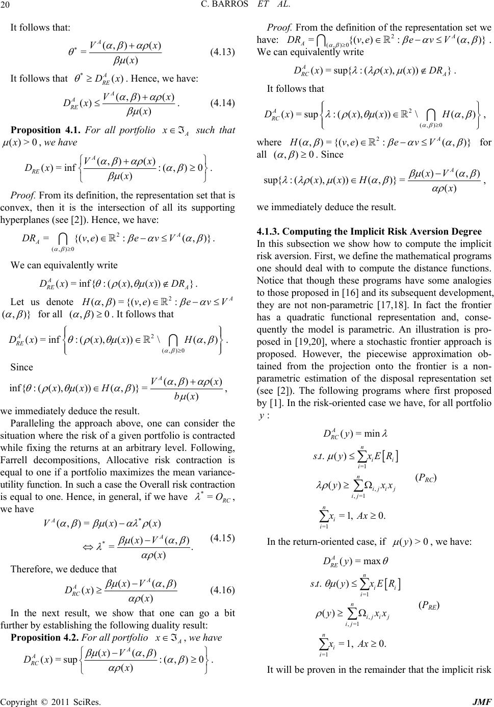

20 C. BARROS ET AL.
It follows that:
(, )()
=()
A
V
x
 

x
(4.13)
It follows that . Hence, we have:
*() A
RE
Dx  
(, )()
() ()
A
A
RE V
Dx x
 


x
. (4.14)
Proposition 4.1. For all portfolio such that
A
x
()>0x

, we have
(, )()
()=inf:( ,)0
()
A
RE Vx
Dx x
 

 



)}
.
Proof. From its definition, the representation set that is
convex, then it is the intersection of all its supporting
hyperplanes (see [2]). Hence, we have:
2
(,)0
={(,): (,
A
A
DRv eevV






 .
We can equivalently write
()=inf{ :( (),())}
A
R
E
Dxxx DR   A .
Let us denote 2 (, )={(,):A
H
veev V   
(, )}

for all (, )0

. It follows that
2
(,)0
()=inf:( (),())\( ,)
A
RE
Dxx xH


















.
Since
(, )()
inf{: ((),())(,)} =()
A
V
xxH bx
 
 

x
,
we immediately deduce the result.
Paralleling the approach above, one can consider the
situation where the risk of a given portfolio is contracted
while fixing the returns at an arbitrary level. Following,
Farrell decompositions, Allocative risk contraction is
equal to one if a portfolio maximizes the mean variance-
utility function. In such a case the Overall risk contraction
is equal to one. Hence, in general, if we have *=
R
C
O  ,
we have
*
*
( ,)=()()
()( ,)
=.
()
A
A
Vxx
xV
x
 







(4.15)
Therefore, we deduce that
()( ,)
() ()
A
A
RC xV
Dx x





 (4.16)
In the next result, we show that one can go a bit
further by establishing the following duality result:
Proposition 4.2. For all portfolio , we have
A
x
()( ,)
()=sup:( ,)0
()
A
A
RC xV
Dx x
 

 


)}
.
Proof. From the definition of the representation set we
have: (,)0
2
={(,): (,
A
A
DRveevV






.
We can equivalently write
()=sup{ :((),())}
A
R
CA
Dxxx DR   .
It follows that
2
(,)0
()=sup:( (),())\( ,)
A
RC
DxxxH

















,
where 2 (, )={(,):(, )}
A
HveevV

 
) 0
 for
all (,

. Since
()( ,)
sup{:(( ),( ))(,)}=()
A
xV
xxH x



 

,
we immediately deduce the result.
4.1.3. Computing the Implicit Risk Aversion Degree
In this subsection we show how to compute the implicit
risk aversion. First, we define the mathematical programs
one should deal with to compute the distance functions.
Notice that though these programs have some analogies
to those proposed in [16] and its subsequent development,
they are not non-parametric [17,18]. In fact the frontier
has a quadratic functional representation and, conse-
quently the model is parametric. An illustration is pro-
posed in [19,20], where a stochastic frontier approach is
proposed. However, the piecewise approximation ob-
tained from the projection onto the frontier is a non-
parametric estimation of the disposal representation set
(see [2]). The following programs where first proposed
by [1]. In the risk-oriented case we have, for all portfolio
:
y

=1
,
,=1
=1
() = min
.. ()
()
=1, 0.
A
RC
n
ii
i
n
ij ij
ij
n
i
i
Dy
s
ty xER
yx
xAx
x









(PRC)
In the return-oriented case, if ()>0y

, we have:

=1
,
,=1
=1
() = max
.. ()
()
=1, 0.
A
RE
n
ii
i
n
ij ij
ij
n
i
i
Dy
s
ty xER
yxx
xAx









(PRE)
It will be proven in the remainder that the implicit risk

C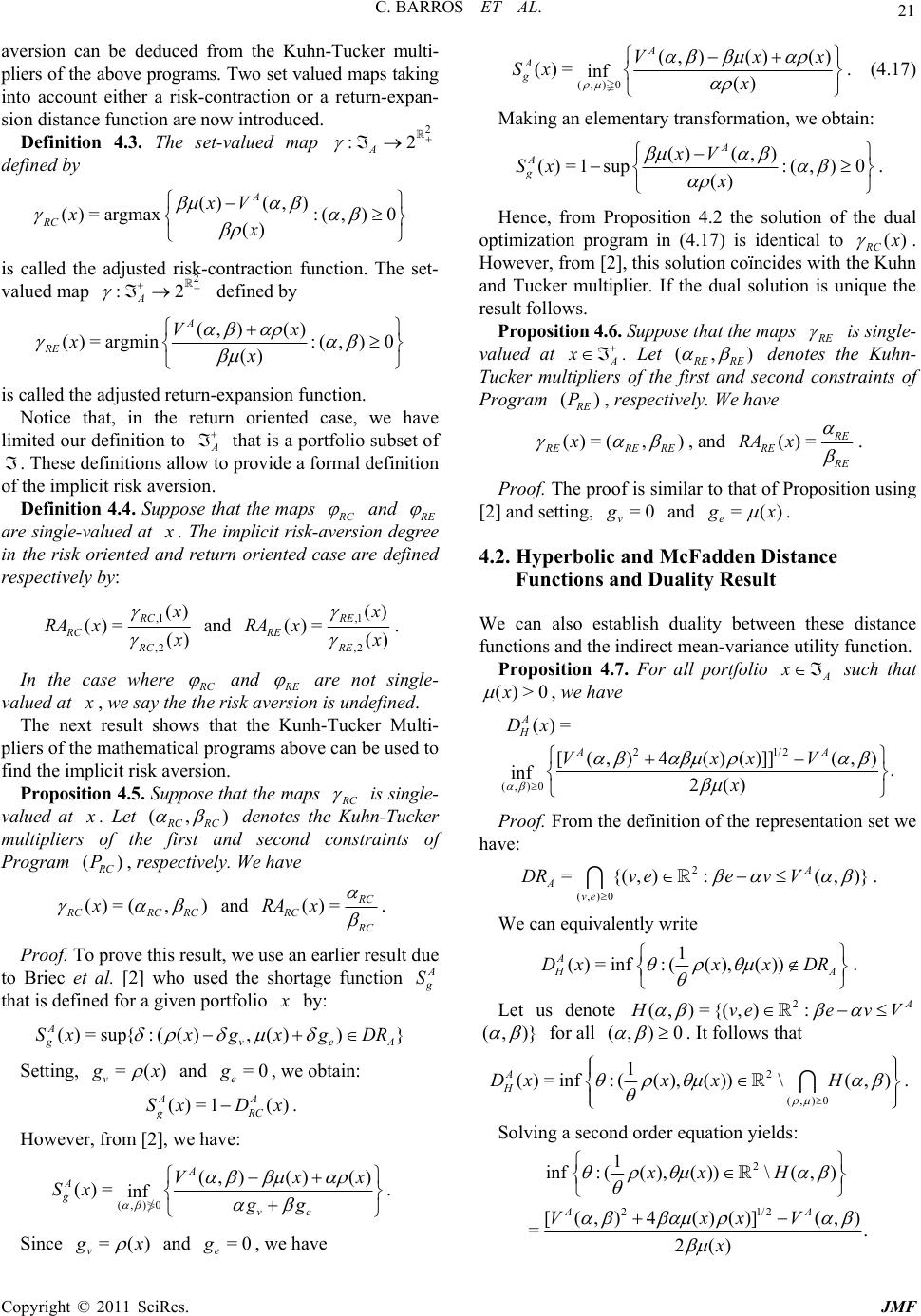. BARROS ET AL.
21
aversion can be deduced from the Kuhn-Tucker multi-
pliers of the above programs. Two set valued maps taking
into account either a risk-contraction or a return-expan-
sion distance function are now introduced.
Definition 4.3. The set-valued map 2
:2
A



defined by
()( ,)
()=argmax:(,)0
()
A
RC xV
xx
 






 


is called the adjusted risk-contraction function. The set-
valued map defined by
2
:2
A



(, )()
()=argmin:( ,)0
()
A
RE Vx
xx
 


 


is called the adjusted return-expansion function.
Notice that, in the return oriented case, we have
limited our definition to A that is a portfolio subset of
. These definitions allow to provide a formal definition
of the implicit risk aversion.



Definition 4.4. Suppose that the maps
R
C

and
R
E

are single-valued at
x
. The implicit risk-aversion degree
in the risk oriented and return oriented case are defined
respectively by:
,1
,2
()
()= ()
RC
RC RC
x
RA x
x


and ,1
,2
()
()= ()
RE
RE RE
x
RA x
x


.
In the case where
R
C

and
R
E

are not single-
valued at
x
, we say the the risk aversion is undefined.
The next result shows that the Kunh-Tucker Multi-
pliers of the mathematical programs above can be used to
find the implicit risk aversion.
Proposition 4.5. Suppose that the maps
R
C

is single-
valued at
x
. Let (,)
R
CRC

denotes the Kuhn-Tucker
multipliers of the first and second constraints of
Program ()
R
C
P, respectively. We have
()=(,)
R
CRC
xRC



and ()=
R
C
RC
R
C
RA x


.
Proof. To prove this result, we use an earlier result due
to Briec et al. [2] who used the shortage function A
g
S
that is defined for a given portfolio
x
by:
()=sup{:( (),())}
A
g
ve
Sxxgxg DR  
A
Setting, =()
v
g
x

and , we obtain: =0
e
g
()=1 ()
AA
gR
SxD xC .
However, from [2], we have:
(,)0
(, )()()
()= inf
A
A
gve
Vx
Sx gg

 







x
.
Since =()
v
g
x

and , we have =0
e
g
(,)0
(, )()()
()= inf ()
A
A
gVx
Sx x

 

x

 




. (4.17)
Making an elementary transformation, we obtain:
()( ,)
()=1sup:( ,)0
()
A
A
gxV
Sx x
 








.
Hence, from Proposition 4.2 the solution of the dual
optimization program in (4.17) is identical to ()
RC
x

.
However, from [2], this solution coïncides with the Kuhn
and Tucker multiplier. If the dual solution is unique the
result follows.
Proposition 4.6. Suppose that the ma ps
R
E

is single-
valued at A
x


. Let (,)
R
ERE

denotes the Kuhn-
Tucker multipliers of the first and second constraints of
Program ()
R
E
P, respectively. We have
()=(,)
R
ERE
xRE



, and ()=
R
E
RE
R
E
RA x


.
Proof. The proof is similar to that of Proposition using
[2] and setting, and
=0
v
g=()
e
g
x

.
4.2. Hyperbolic and McFadden Distance
Functions and Duality Result
We can also establish duality between these distance
functions and the indirect mean-variance utility function.
Proposition 4.7. For all portfolio such that
A
x
()>0x

, we have
21/2
(,)0
()=
[(,) 4()()]](,)
.
inf 2()
A
H
AA
Dx
VxxV
x

 








Proof. From the definition of the representation set we
have:
2
(,)0
={(,):(,)
A
Ave
DRv eevV}




.
We can equivalently write
1
()=inf:((), ())
A
HA
Dxxx DR 







.
Let us denote 2 (, )={(,):A
H
veev V   
(, )}

for all (, )0

. It follows that
2
(,)0
1
()=inf:((),())\( ,)
A
H
Dxx xH


















.
Solving a second order equation yields:
2
21/2
1
inf:((),())\(,)
[(,)4 ()()](,)
=.
2()
AA
xx H
VxxV
x
 


 










C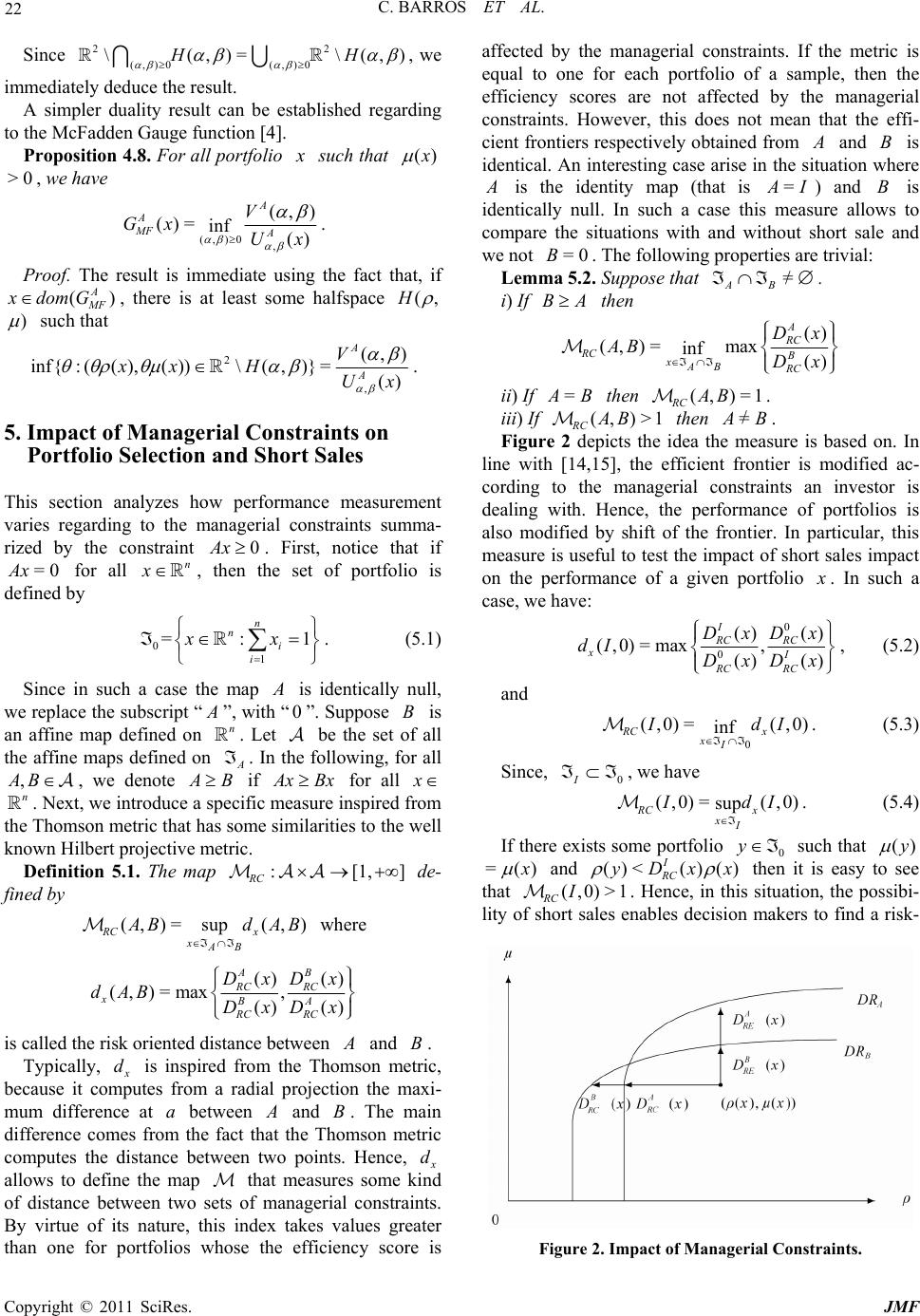. BARROS ET AL.
22
2
,)H
Since 2
(,)0 (,)0
\(,)= \(H
 





 
, we
immediately deduce the result.
A simpler duality result can be established regarding
to the McFadden Gauge function [4].
Proposition 4.8. For all portfolio
x
such that ()
x

, we have >0
(,)0,
(,)
()= inf ()
A
A
MF A
V
Gx Ux
 


.
Proof. The result is immediate using the fact that, if
(
A)
M
F
xdom G, there is at least some halfspace (,H

)

such that
2
,
(,)
inf{: ((),())\(,)} =()
A
A
V
xx HUx



  .
5. Impact of Managerial Constraints on
Portfolio Selection and Short Sales
This section analyzes how performance measurement
varies regarding to the managerial constraints summa-
rized by the constraint . First, notice that if
for all , then the set of portfolio is
defined by
0Ax 
=0Ax n
x
0
1
=:
n
ni
i
xx


 



1


. (5.1)
Since in such a case the map
A
is identically null,
we replace the subscript “
A
”, with “”. Suppose is
an affine map defined on . Let be the set of all
the affine maps defined on A. In the following, for all
, we denote
0

B
n


,AB
A
B if
A
xBx for all
x

. Next, we introduce a specific measure inspired from
the Thomson metric that has some similarities to the well
known Hilbert projective metric.
n

Definition 5.1. The map de-
fined by :[1,
RC ]
(, )=(,)
sup
RC x
xAB
A
Bd
 
AB where
() ()
(,)=max ,
() ()
AB
RC RC
xBA
RC RC
DxDx
dAB DxDx





is called the risk oriented distance between
A
and .
B
Typically,
x
d is inspired from the Thomson metric,
because it computes from a radial projection the maxi-
mum difference at a between
A
and . The main
difference comes from the fact that the Thomson metric
computes the distance between two points. Hence,
B
x
d
allows to define the map that measures some kind
of distance between two sets of managerial constraints.
By virtue of its nature, this index takes values greater
than one for portfolios whose the efficiency score is
affected by the managerial constraints. If the metric is
equal to one for each portfolio of a sample, then the
efficiency scores are not affected by the managerial
constraints. However, this does not mean that the effi-
cient frontiers respectively obtained from

A
and is
identical. An interesting case arise in the situation where
B
A
is the identity map (that is =
A
I

) and is
identically null. In such a case this measure allows to
compare the situations with and without short sale and
we not . The following properties are trivial:
B
=0B
BA 
Lemma 5.2. Suppose that . =
AB
 
i) If then
()
()
Dx
Dx





(, )= ma
inf
xAB
AB x
A
RC
B
RC
RC

= ii) If
A
B

then . (, )=
RC AB
>1 =
1
iii) If then (,)AB
RC
A
B .
Figure 2 depicts the idea the measure is based on. In
line with [14,15], the efficient frontier is modified ac-
cording to the managerial constraints an investor is
dealing with. Hence, the performance of portfolios is
also modified by shift of the frontier. In particular, this
measure is useful to test the impact of short sales impact
on the performance of a given portfolio
x
. In such a
case, we have:
0
,RC
I
RC
0
()
(,0)=max ()
I
RC
RC
Dx
dI Dx
()
()
Dx
Dx
x









)
, (5.2)
and
0
(,0)=inf
RC xI
(,0
x
I
dI
 
. (5.3)
Since, 0I

 , we have
(,0)=
sup
RC x
xI
(,0)
I
dI


. (5.4)
If there exists some portfolio 0 such that y()y

=()
x

and ()< ()(
I
RC )
y
Dx 
)>1
x  then it is easy to see
that RC. Hence, in this situation, the possibi-
lity of short sales enables decision makers to find a risk-
(,0I
Figure 2. Impact of Managerial Constraints.

C. BARROS ET AL.
23
]
less portfolio. A similar approach is possible when one
looks for possible improvement of the return.
Definition 5.3. The map de-
fined by :[1,
RC 
(, )=(, )
sup
RE x
xAB
A
BAB


 
 where
() ()
(, )=max,
() ()
AB
RE RE
xBA
RE RE
DxDx
AB DxDx 





(5.5)
is called the risk oriented distance between
A
and . B
Lemma 5.4. The following properties are also trivial.
Suppose that =
AB


 
A. i) If then B
()
(,)= max sup ()
B
RE
RE A
xRE
AB
Dx
AB Dx
 




ii) If =
A
B

then . (, )=1
RE AB
>1 = iii) If then (, )AB
RE
A
B
.
This measure is useful to test whether or not the short
sales impact the return expansion given some portfolio
x
. In such a case, we have:
0
0
() ()
(,0)=max ,
() ()
I
RE RE
xI
RE RE
DxDx
IDxDx 



, (5.6)
and since, , we have
0I

(,0)=(,0)
sup
RE x
xI
I
I


. (5.7)
If there exists some portfolio 0 such that y ()y

=()
x

and , then it is easy to see
that RC. Hence, in this situation, the possibi-
lity of short sales enables decision makers to find a
riskless portfolio.
() ()<(
I
RE
Dx x 
0)>1
)y 
(,I
In general, it is difficult to compute the map (,
RE
A

and )B(,)
RC
A
B. However, one can compute an
approximation based upon each specific asset. By
construction, we have i
, for where
=1, ,n is the canonical basis of . This we do by
defining
()=
i
Re R=1,i
n,n
{}
ii
e
1, ,
(,0) max(,0)i
RC e
in
I
dI


 and (5.8)
1, ,
(,0) max(,0)i
RE e
in
I
I 


. (5.9)
To analyse the case where there are short sales, an
approach based upon quadratic programming may be
used. However, since the optimization constraints are
binding, it is possible to give a solution in closed form
for *

, *

and *
x
.
6. Empirical Illustration
This section presents a numerical example. It is shown
that some key contributions of this paper can be easily
implemented using standard methods of quadratic pro-
gramming. The data are obtained from the CAC 40
monthly stocks over a period running from January 1984
to December 2008. For each of the 38 stocks, we have
calculated monthly expected returns, covariances, varian-
ces with a monthly percentage return. After computing
the efficient frontier, we set parameters =1

and =

. Below, Tables 1 and 2 respectively summarize in the
risk oriented and return oriented cases the decompo-
sition of monthly performances for each asset. Remember
that overall efficiency looks for a global improvement of
a title following a chosen direction. Hence, it can be
decomposed in two parts reflecting portfolio efficiency
and allocative efficiency.
2
As it is shown in Table 1, asset 1 (Accor) has a low
return and therefore it is too risky. The investor can
Table 1. Decomposition of “CAC 40” performance (Risk
Oriented).
Asset
R
C
O
R
C
D
R
C
A
R
C

Accor 2.9767 0.0358 2.9409 0.0000
Air france 0.8191 0.0291 0.7900 0.0140
Air liquide 9.6218 0.0935 9.5283 0.0000
Alcaltel –0.1972 0.2086 –0.4058 0.0133
Alstom –0.6221 1.0000 –1.6221 0.0196
Arcelor mittal3.6585 0.0438 3.6147 0.0000
Axa 1.8391 0.0225 1.8166 0.0000
Bnp 2.5783 0.0336 2.5447 0.0000
Bouygues 2.6120 0.0269 2.5851 0.0000
Cap gemini 0.5518 0.0147 0.5372 0.0230
Carrefour 5.0090 0.0489 4.9601 0.0000
Credit agricole2.1384 0.1024 2.0360 0.0097
Danone 6.1840 0.0623 6.1218 0.0000
Dexia –0.1622 0.3111 –0.4733 0.0128
Eads 1.2664 0.0392 1.2272 0.0175
Edf 17.4122 0.1721 17.2401 0.0000
Essilor intl 9.2642 0.0716 9.1925 0.0000
France telecom0.1872 0.0333 0.1539 0.0107
Gdf suez 41.1744 0.3918 40.7825 0.0000
Lafarge 2.5799 0.0362 2.5437 0.0000
Lagardere 2.3142 0.0272 2.2869 0.0000
Loreal 6.2259 0.0522 6.1737 0.0000
Lvmh 2.4824 0.0286 2.4539 0.0000
Michelin 2.6201 0.0354 2.5847 0.0000
Pernod ricard6.5931 0.0642 6.5289 0.0000
Peugeot 1.8569 0.0284 1.8285 0.0000
Ppr 2.1359 0.0258 2.1101 0.0000
Renault 0.9004 0.0209 0.8794 0.0319
Saint gobain2.7787 0.0324 2.7463 0.0000
Sanofi aventis9.4330 0.1144 9.3185 0.0000
Schneider 3.0940 0.0356 3.0584 0.0000
Societe generale2.2684 0.0269 2.2415 0.0000
Stmicroelec-
tronics 0.9322 0.0161 0.9161 0.1430
Suez E. 15.3026 0.9597 14.3429 0.0071
Total 7.2215 0.0662 7.1553 0.0000
Unibail 5.4427 0.0559 5.3868 0.0000
Vallourec 2.1729 0.0181 2.1548 0.0000
Veolia environ2.1113 0.0484 2.0628 0.0337
Vinci 3.9696 0.0393 3.9303 0.0000
Vivendi 1.8895 0.0288 1.8607 0.0000

24 C. BARROS ET AL.
Table 2. Decomposition of “CAC 40” performance (Return
Oriented).
Asset
R
E
O
R
E
D
R
E
A
R
E

Accor 33.6665 33.6640 0.0025 0.0133
Air france 2.5886 2.5561 0.0325 0.0135
Air liquide –5.8125 –5.5131 –0.2994 0.0128
Alcaltel 1.8827 1.5611 0.3215 0.0170
Alstom 1.3252 1.0000 0.3252 0.0196
Arcelor mittal 37.7219 37.5822 0.1397 0.0132
Axa 27.2942 26.9360 0.3582 0.0135
Bnp 11.8982 11.8983 –0.0001 0.0133
Bouygues –11.7382 –11.6888 –0.0494 0.0134
Cap gemini 3.7739 3.4874 0.2865 0.0142
Carrefour –6.6492 –6.5984 –0.0508 0.0132
Credit agricole 1.7816 1.7288 0.0528 0.0130
Danone –7.8429 –7.6831 –0.1599 0.0131
Dexia 1.3169 1.3140 0.0030 0.0134
Eads 2.4821 2.4815 0.0005 0.0134
Edf –6.1239 –5.4436 –0.6804 0.0122
Essilor intl –2.3266 –2.2569 –0.0697 0.0130
France telecom 2.3786 2.1740 0.2046 0.0147
Gdf suez –4.6683 –3.7145 –0.9538 0.0103
Lafarge 7.5510 7.5500 0.0010 0.0133
Lagardere 77.9918 77.6968 0.2950 0.0134
Loreal –3.2041 –3.1702 –0.0339 0.0132
Lvmh –307.6488 –306.9223 –0.7265 0.0134
Michelin 9.2097 9.2095 0.0001 0.0133
Pernod ricard –6.2128 –6.0738 –0.1390 0.0130
Peugeot 5.7738 5.7592 0.0146 0.0134
Ppr 33.6970 33.4996 0.1974 0.0134
Renault 3.4948 3.4060 0.0888 0.0135
Saint gobain 162.9716 162.9394 0.0322 0.0134
Sanofi aventis 25.2989 23.5278 1.7711 0.0126
Schneider –252.3979 –252.3878 –0.0100 0.0133
Societe
generale 56.2202 55.9829 0.2373 0.0134
Stmicroelec-
tronics 5.2064 4.9761 0.2303 0.0136
Suez
environnement 1.4416 1.0284 0.4132 0.0037
Total –4.4442 –4.3357 –0.1085 0.0130
Unibail –9.4252 –9.2927 –0.1325 0.0131
Vallourec –4.2453 –4.1137 –0.1315 0.0135
Veolia environ 2.7819 2.7700 0.0119 0.0132
Vinci –7.6228 –7.6144 –0.0085 0.0133
Vivendi 5.8051 5.7926 0.0125 0.0134
choose an efficient portfolio that is less risky
and does not require risk-taking (
0,0 36%
=0
RC

). Considering
only risk aversion, it is possible to pursue reduction of
risk to maximize the utility of a portfolio but, due to the
market imperfections, this result cannot be achieved
without short sales.
In the return expansion case, the first asset is less
efficient (Table 2) than is the risk oriented case. Given
the same level of risk, it should be 50 times more
profitable (). However, technically, we
can only select a portfolio that produces 33 times more
important return (). The market imperfec-
tions again limits this return improvement ().
Here, the investor must take 6 units of risk to increase his
(or her) return of a one unit amount (
= 33.6665
RE
O
= 3
RE
D3.6641
= 0.0025
RE
A
= 0.0133
RE

).
Table 3 details implicit risk aversion of risk reduction
Table 3. Implicit Risk Aversion.
Asset Risk Oriented Return Oriented
R
C

R
C

R
C

R
E

R
E

R
E

Accor 0.000 1.000 0.000 0.006 0.482 0.013
Air france0.000 0.011 0.014 0.008 0.613 0.013
Air liquide0.000 1.000 0.000 0.003 0.284 0.012
Alcaltel 0.006 0.462 0.013 0.020 1.197 0.017
Alstom 0.030 1.534 0.019 0.030 1.534 0.019
Arcelor mittal0.0001.000 0.000 0.005 0.4330.013
Axa 0.000 1.000 0.000 0.008 0.616 0.013
Bnp 0.000 1.000 0.000 0.006 0.499 0.013
Bouygues 0.000 1.000 0.000 0.007 0.5610.013
Cap gemini0.000 0.008 0.023 0.012 0.8460.014
Carrefour 0.000 1.000 0.000 0.005 0.4080.013
Credit agricole0.000 0.014 0.009 0.004 0.3320.013
Danone 0.000 1.000 0.000 0.004 0.358 0.013
Dexia 0.003 0.287 0.012 0.007 0.542 0.013
Eads 0.000 0.010 0.017 0.006 0.5090.013
Edf 0.000 1.000 0.000 0.002 0.195 0.012
Essilor intl0.000 1.000 0.000 0.004 0.331 0.013
France
telecom 0.001 0.105 0.010 0.013 0.890 0.014
Gdf suez 0.000 1.000 0.000 0.001 0.095 0.010
Lafarge 0.000 1.000 0.000 0.006 0.480 0.013
Lagardere 0.000 1.000 0.000 0.007 0.557 0.013
Loreal 0.000 1.000 0.000 0.005 0.394 0.013
Lvmh 0.000 1.000 0.000 0.007 0.5430.013
Michelin 0.000 1.000 0.000 0.006 0.485 0.013
Pernod ricard0.000 1.000 0.000 0.004 0.352 0.013
Peugeot 0.000 1.000 0.000 0.007 0.5450.013
Ppr 0.000 1.000 0.000 0.007 0.573 0.013
Renault 0.000 0.006 0.031 0.009 0.668 0.013
Saint gobain0.000 1.000 0.000 0.006 0.5090.013
Sanofi aventis0.000 1.000 0.000 0.003 0.252 0.012
Schneider 0.000 1.000 0.000 0.006 0.484 0.013
Societe
generale 0.000 1.000 0.000 0.007 0.561 0.013
Stmicroelec-
tronics 0.000 0.001 0.143 0.009 0.7330.013
Suez E. 0.000 0.017 0.007 0.000 0.021 0.003
Total 0.000 1.000 0.000 0.004 0.346 0.013
Unibail 0.000 1.000 0.000 0.005 0.380 0.013
Vallourec 0.000 1.000 0.000 0.009 0.689 0.013
Veolia environ0.000 0.006 0.033 0.005 0.429 0.013
Vinci 0.000 1.000 0.000 0.006 0.459 0.013
Vivendi 0.000 1.000 0.000 0.007 0.5410.013
and return expansion for each asset. Note that some
assets have a negative performance indicator. This can be
explained by the fact that they have a negative return.
The portfolio may have a greater risk than their expected
returns and their respective utility functions measures the
potential loss of each invested euro. This is not consistent
with the objective of maximizing behaviour the investors
have and, in such a case, allocative efficiency makes no
sense.
Improvements both based on increasing expected
returns and risk contraction are presented in Table 4. In
general, the shortage function and the hyperbolic function
give almost the same improvement of performance
(0.008 for asset 1). The Hyperbolic functions provide a
seven times greater improvement than those obtained
from these two functions. Hence, much more return, but

C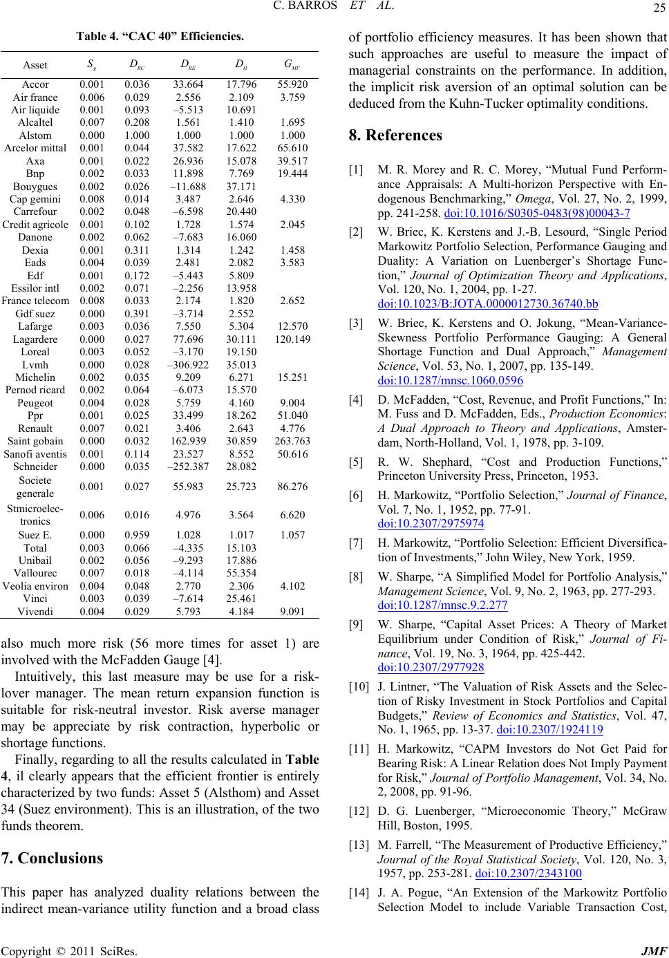. BARROS ET AL.
25
Table 4. “CAC 40” Efficiencies.
Asset
g
S
R
C
D
R
E
D
H
D
M
F
G
Accor 0.001 0.036 33.664 17.796 55.920
Air france 0.006 0.029 2.556 2.109 3.759
Air liquide 0.001 0.093 –5.513 10.691
Alcaltel 0.007 0.208 1.561 1.410 1.695
Alstom 0.000 1.000 1.000 1.000 1.000
Arcelor mittal 0.001 0.044 37.582 17.622 65.610
Axa 0.001 0.022 26.936 15.078 39.517
Bnp 0.002 0.033 11.898 7.769 19.444
Bouygues 0.002 0.026 –11.688 37.171
Cap gemini 0.008 0.014 3.487 2.646 4.330
Carrefour 0.002 0.048 –6.598 20.440
Credit agricole 0.001 0.102 1.728 1.574 2.045
Danone 0.002 0.062 –7.683 16.060
Dexia 0.001 0.311 1.314 1.242 1.458
Eads 0.004 0.039 2.481 2.082 3.583
Edf 0.001 0.172 –5.443 5.809
Essilor intl 0.002 0.071 –2.256 13.958
France telecom 0.008 0.033 2.174 1.820 2.652
Gdf suez 0.000 0.391 –3.714 2.552
Lafarge 0.003 0.036 7.550 5.304 12.570
Lagardere 0.000 0.027 77.696 30.111 120.149
Loreal 0.003 0.052 –3.170 19.150
Lvmh 0.000 0.028 –306.922 35.013
Michelin 0.002 0.035 9.209 6.271 15.251
Pernod ricard 0.002 0.064 –6.073 15.570
Peugeot 0.004 0.028 5.759 4.160 9.004
Ppr 0.001 0.025 33.499 18.262 51.040
Renault 0.007 0.021 3.406 2.643 4.776
Saint gobain 0.000 0.032 162.939 30.859 263.763
Sanofi aventis 0.001 0.114 23.527 8.552 50.616
Schneider 0.000 0.035 –252.387 28.082
Societe
generale 0.001 0.027 55.983 25.723 86.276
Stmicroelec-
tronics 0.006 0.016 4.976 3.564 6.620
Suez E. 0.000 0.959 1.028 1.017 1.057
Total 0.003 0.066 –4.335 15.103
Unibail 0.002 0.056 –9.293 17.886
Vallourec 0.007 0.018 –4.114 55.354
Veolia environ 0.004 0.048 2.770 2.306 4.102
Vinci 0.003 0.039 –7.614 25.461
Vivendi 0.004 0.029 5.793 4.184 9.091
also much more risk (56 more times for asset 1) are
involved with the McFadden Gauge [4].
Intuitively, this last measure may be use for a risk-
lover manager. The mean return expansion function is
suitable for risk-neutral investor. Risk averse manager
may be appreciate by risk contraction, hyperbolic or
shortage functions.
Finally, regarding to all the results calculated in Table
4, il clearly appears that the efficient frontier is entirely
characterized by two funds: Asset 5 (Alsthom) and Asset
34 (Suez environment). This is an illustration, of the two
funds theorem.
7. Conclusions
This paper has analyzed duality relations between the
indirect mean-variance utility function and a broad class
of portfolio efficiency measures. It has been shown that
such approaches are useful to measure the impact of
managerial constraints on the performance. In addition,
the implicit risk aversion of an optimal solution can be
deduced from the Kuhn-Tucker optimality conditions.
8. References
[1] M. R. Morey and R. C. Morey, “Mutual Fund Perform-
ance Appraisals: A Multi-horizon Perspective with En-
dogenous Benchmarking,” Omega, Vol. 27, No. 2, 1999,
pp. 241-258. doi:10.1016/S0305-0483(98)00043-7
[2] W. Briec, K. Kerstens and J.-B. Lesourd, “Single Period
Markowitz Portfolio Selection, Performance Gauging and
Duality: A Variation on Luenberger’s Shortage Func-
tion,” Journal of Optimization Theory and Applications,
Vol. 120, No. 1, 2004, pp. 1-27.
doi:10.1023/B:JOTA.0000012730.36740.bb
[3] W. Briec, K. Kerstens and O. Jokung, “Mean-Variance-
Skewness Portfolio Performance Gauging: A General
Shortage Function and Dual Approach,” Management
Science, Vol. 53, No. 1, 2007, pp. 135-149.
doi:10.1287/mnsc.1060.0596
[4] D. McFadden, “Cost, Revenue, and Profit Functions,” In:
M. Fuss and D. McFadden, Eds., Production Economics:
A Dual Approach to Theory and Applications, Amster-
dam, North-Holland, Vol. 1, 1978, pp. 3-109.
[5] R. W. Shephard, “Cost and Production Functions,”
Princeton University Press, Princeton, 1953.
[6] H. Markowitz, “Portfolio Selection,” Journal of Finance,
Vol. 7, No. 1, 1952, pp. 77-91.
doi:10.2307/2975974
[7] H. Markowitz, “Portfolio Selection: Efficient Diversifica-
tion of Investments,” John Wiley, New York, 1959.
[8] W. Sharpe, “A Simplified Model for Portfolio Analysis,”
Management Science, Vol. 9, No. 2, 1963, pp. 277-293.
doi:10.1287/mnsc.9.2.277
[9] W. Sharpe, “Capital Asset Prices: A Theory of Market
Equilibrium under Condition of Risk,” Journal of Fi-
nance, Vol. 19, No. 3, 1964, pp. 425-442.
doi:10.2307/2977928
[10] J. Lintner, “The Valuation of Risk Assets and the Selec-
tion of Risky Investment in Stock Portfolios and Capital
Budgets,” Review of Economics and Statistics, Vol. 47,
No. 1, 1965, pp. 13-37. doi:10.2307/1924119
[11] H. Markowitz, “CAPM Investors do Not Get Paid for
Bearing Risk: A Linear Relation does Not Imply Payment
for Risk,” Journal of Portfolio Management, Vol. 34, No.
2, 2008, pp. 91-96.
[12] D. G. Luenberger, “Microeconomic Theory,” McGraw
Hill, Boston, 1995.
[13] M. Farrell, “The Measurement of Productive Efficiency,”
Journal of the Royal Statistical Society, Vol. 120, No. 3,
1957, pp. 253-281. doi:10.2307/2343100
[14] J. A. Pogue, “An Extension of the Markowitz Portfolio
Selection Model to include Variable Transaction Cost,

C. BARROS ET AL.
26
short Sales, Leverage Polycies and Taxes,” Journal of
Finance, Vol. 25, No. 5, 1970, pp. 1005-1028.
doi:10.2307/2325576
[18] R. Färe, S. Grosskopf, C. A. K. Lovell, “The Measure-
ment of Efficiency of Production,” Kluwer, Boston, 1985.
[19] W. Briec and J.-B. Lesourd, “The Efficiency of Invest-
ment Fund Management: A Stochastic Frontier Model,”
In: Dunis, Eds., Advances in Quantitative Asset Man-
agement, Klwer Academic Publishers, Norwell. 2000, pp.
41-58.
[15] A. Rudd and B. Rosenberg, “A Realistic Portfolio Selec-
tion Model,” In: E. J. Elton and M. J. Grubber, Eds.,
Portfolio Theory-Lectures in Management Science, Vol.
II, North Holland, Amsterdam, 1979, pp. 21-46.
[20] A. Ruszczynski and R. Vanderbei, “Frontiers of Stochas-
tically Nondominated Portfolios,” Econometrica, Vol. 71,
No. 4, 2003, pp. 1287-1297.
doi:10.1111/1468-0262.t01-1-00448
[16] A. Charnes, W. W. Cooper and E. Rhodes, “Measuring
the Efficiency of Decision-Making Units,” European
Journal of Operational Research, Vol. 3, No. 6, 1978, pp.
429-444. doi:10.1016/0377-2217(78)90138-8
[17] J. K. Sengupta, “Nonparametric Tests of Efficiency of
Portfolio Investment,” Journal of Economics, Vol. 50, No.
1, 1989, pp. 1-15. doi:10.1007/BF01227605
[21] A. V. Fiacco and G. P. McGormick, “Nonlinear Pro-
gramming: Sequential Uncontrained Minimization Tech-
niques,” John Wiley, New York, 1968.
Appendix: The Short Sale Case
Computations 1 =1[
n]
x
ER








Ω (7.4)
Since the constraints are binding.
It is possible to give a solution of the case where there
are short sales with an approach based upon quadratic
programming.
#
[()][( )]ERx ERx
Hence, substituting in the first order conditions, we have
a three-dimensional system to solve, with:
Computation of Risk Oriented Measure [] 1[]=0
tnp
ERERE R








(7.5)
In the following, we assume that # ()( )
x
x  
))x
where
. Under such an assumption,
we know that RC lies on the curve
representing the hyperbola relating the expected returns
and the variance. We first write the Lagrangian of the
optimization problem we need to solve. It is defined by
#
0
argmin{() :}xxx  
0
(()Dx
1
1[]1[]=
tnn
ERERV R
 
 







Ω


(
Suppose that
(),(x 
0
p
(7.6)
1
11[]
tnn
ER






Ω =1

(7.7)
The last equation yields:

,
,
(,,,, )=
1
ii p
i
pijiji
ij i
LxxERE R
VarRx xx
 
 












 



7.1)

1
1
1
=1
11
tn
tnn
ER








Ω
Ω
[] (7.8)
Substituting in 7.5, we obtain:
** ***
(,,, ,)x

 is solution. The fi
order conditions yield:
rst


1
1
1
1
[]1 1[]1
11
[]=0.
tt
nnn
tnn
p
ER ER
ERE R
















Ω
Ω
Ω

,
(,,,, )==0
ijij
j
i
LxER x
x
 

 (7.2)
(,,,, )=1[]=0
p
Lx VarR  


 (7.3)
Following (7.2); we have Hence, we obtain the optimal values:

C. BARROS ET AL.
27

*
1
=[ []1[]1[]
tt t
ERER ER


ΩΩ
1 1
*
1
[]]
1
[[]1]
11
nn
tnp
tnn
ER
ERE R









Ω
(7.9)
and *

ce
is then obtained from equation 46. From 52, we
dedu *
x
. The distance function is given by *

*1
1
=[] 1
1
11
p
n
tnn



Ω Var R



**
11
**
*
1
1*
*
1
*
1[]1[]
1
11[]1
11
[].
tnn
t
nn
tnn
ER ER
ER
ER






















ΩΩ
ΩΩ
Ω
Ω
n
(7.10)
Computation of Return Oriented Measure
The




(7.11)
Suppose that
In the following, we suppose that [] >0 ER
p.
em we neLagrangian of the optimization probled to
optimize is:
(, ,,,Lx 

,
,
)=
1
ii p
i
pijij i
ij i
xERE R
VarRx xx
 



 









 



** ***
(,,, ,)x

 is solution. The first
order conditions yield:

,
(,,,, )=LxE  
=0
ijij
j
i
R x
x
   
 (7.12)

(,,,, )==0
i
i
Lx ER
x


 (7.13)
(,,,, )=1[]=0
p
Lx ER  



*
(7.14)
At the optimum, we clearly have =1/[]
p
ER . 
Following (7.2); we have
1
=1[]
n
x
ER




(7.14)
Since the constraints are binding, substituting in the
first order conditions, we have a three-d
te



Ω
imensional sys-
m to solve, with:
[] 1[]=0
tn
ERERE R
 





 (7.15)
p



1
1[]1[
=0
tnn
p
ER ER
Var R
 
 


]


 
Ω
(7.16)


1
11[]
tnn
ER






Ω =1 (7.17)
Combining 7.15 and 7.16 we obtain




2
1[] =0
tpp
 p
ERERER VarR 

   Ω (7.18)
It follows that
*1/2
1/2
=[ ]
[][]
tpp
p
ER ER
ERVar R


 
 


Ω
1/2
(7.19)
Using 7.17 and 7.15 we obtain:


1
1*
1[]1
[]= 0
n
p
ER
ERE R






1
[] 1 1
11
tt
nn
tnn
ER








Ω
Ω
Hence, we obtain the optimal values:


Ω

*1
*
1
[]
1
[]1.
11
tnp
tnn
ER
ERE R


11
*=[]1[]1[]
tt t
nn
ERERER













 




Ω
(7.20)
Therefore
ΩΩ
*

and *

we de
are then obtained from equa-
tion 7.20. Fr 7.14,duce om*
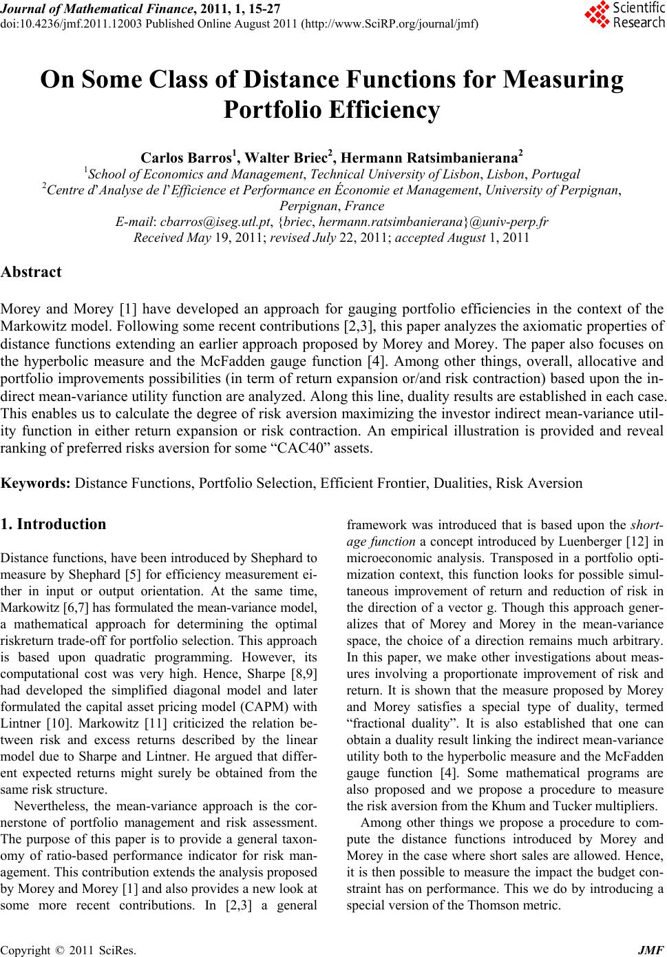
x
.