Journal of Mathematical Finance, 2011, 1, 28-33
doi:10.4236/jmf.2011.12004 Published Online August 2011 (http://www.SciRP.org/journal/jmf)
Option Pricing When Changes of the Underlying Asset
Prices Are Restricted
George J. Jiang1,2, Guanzhong Pan2, Lei Shi 3
1University of Arizona, Tucson, USA
2College of Finance, Yu nn a n Uni versit y of Fi na nce an d Economics, Kunming, China
2College of Statistics and Math ematics, Yunnan University of Finance and Economics, Kunming, China
Received April 8, 2011; revised June 13, 2011; accepted July 10, 2011
Abstract
Exchanges often impose daily limits for asset price changes. These restrictions have a direct impact on the
prices of options traded on these assets. In this paper, we derive closed-form solution of option pricing for-
mula when there are restrictions on changes in underlying asset prices. Using numerical examples, we illus-
trate that very often the impact of such restrictions on option prices is substantial.
Keywords: Option Pricing, Restrictions on Asset Price Changes, Numerical Illustration
1. Introduction
Conventional option pricing models assume that there
are no restrictions on changes of underlying asset prices.
For example, [1,2] specify that stock prices follow a
geometric Brownian motion and stock returns follow a
normal distribution. Based on a portfolio replication
strategy or equivalently the risk-neutral method, option
prices are derived as expected payoff of the contract un-
der the risk-neutral distribution, discounted by the risk-
free rate.
In practice, however, asset price changes may subject
to restrictions imposed by exchanges. For example,
CBOT (Chicago Board of Trade) and CME (Chicago
Mercantile Exchange) both have daily price limits for
futures contracts except currency futures. Daily price
limit serves as a precautionary measure to prevent ab-
normal market movement. The price limits, quoted in
terms of the previous or prior settlement price plus or
minus the specific trading limit, are set based on particu-
lar product specifications. For example, the current limit
of daily price changes on short term corn futures is 4.5%.
In 1996, Chinese stock market also introduces restric-
tions on daily stock price changes. Specifically, except
the first trading day of newly issued stocks, the limit of
stock price change in a trading day relative to previous
day’s close price is 10%, and for stocks that begin with S,
ST, S*ST letters, the limit is 5%. It is clear that such re-
strictions reduce the value of options since extreme re-
turns on a daily level are ruled out. Nevertheless, how to
evaluate the prices of option contracts when changes on
underlying asset prices are restricted? How much is the
exact impact of such daily price limits on option prices?
These questions are yet to be examined in the extant lit-
erature.
In this paper, we first derive the option pricing for-
mula when there are restrictions on daily changes of un-
derlying asset prices. We perform the analysis under the
Black-Scholes-Merton model framework. Then, we pro-
vide numerical comparisons between option prices with
and without restrictions on underlying asset price changes.
2. Option Pricing with Restrictions on
Underlying Asset Price Changes
2.1. Risk-Neutral Valuation under the Black and
Scholes [1] and Merton [2] Framework
In this section, we first review the risk-neutral approach
of option pricing under Black-Scholes-Merton frame-
work. The same approach will be used in the next sub-
section to derive option pricing formula when there are
restrictions on underlying asset price changes. Black and
Scholes [1] and Merton [2] assume that stock price
follows a geometric Brownian motion:
t
S
dd
tt t
SStSd
t
W



 (1)
where

and

are expected return and volatility,
t is a standard Brownian motion. It is also assumed
that the continuously compounded risk-free interest rate,
W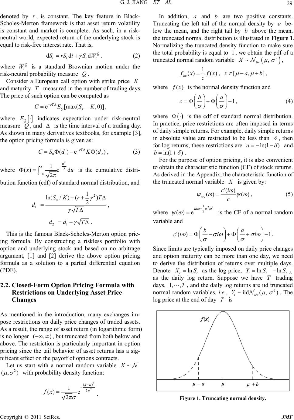

G. J. JIANG ET AL.
29
denoted by , is constant. The key feature in Black-
Scholes-Merton framework is that asset return volatility
is constant and market is complete. As such, in a risk-
neutral world, expected return of the underlying stock is
equal to risk-free interest rate. That is,
r
ddd
Q
tt tt
S rStSW   . (2)
where is a standard Brownian motion under the
risk-neutral probability measure .
Q
t
WQ
Consider a European call option with strike price
K
and maturity measured in the number of trading days.
The price of such option can be computed as
T
e[max(,0
rT QT
CESK

)],
where


Q
EQ indicates expectation under risk-neutral
measure , and is the time interval of a trading day.
As shown in many derivatives textbooks, for example [3],
the option pricing formula is given as:

01 2
()e ()
rT
CS dKd

 , (3)
where
2
2
1
()e d
2π
u
x
x
u



 is the cumulative distri-
bution function (cdf) of standard normal distribution, and
2
0
1
d
1
ln(/) ()
2
SK rT
T


 
 ,
21
dd T   .
This is the famous Black-Scholes-Merton option pric-
ing formula. By constructing a riskless portfolio with
option and underlying stock and based on no arbitrage
argument, [1] and [2] derive the above option pricing
formula as a solution to a partial differential equation
(PDE).
2.2. Closed-Form Option Pricing Formula with
Restrictions on Underlying Asset Price
Changes
As mentioned in the introduction, many exchanges im-
pose restrictions on daily price changes of traded assets.
As a result, the range of asset return (in logarithmic form)
is no longer , but truncated from both below and
above. The restriction is particularly important in option
pricing since the tail behavior of asset returns has a sig-
nificant effect on the payoff of options contracts.
(, )
Let us start with a normal random variable ~X

2
(, )

 with probability density function:
2
2
()
2
1
() e
2π
x
fx





.
In addition, and are two positive constants.
Truncating the left tail of the normal density b a be-
low the mean, and the right tail by b above the mean,
the truncated normal distribution is illustrated in Figure 1 .
Normalizing the truncated density function to make sure
the total probability is equal to , we obtain the pdf of a
truncated normal random variable
ab
y
1

trc
~,X



2

,
trc
1
() ()
f
xf
c
x], [,
x
ab

 ,
where ()
f
x is the normal density function and
1
ba
c

 


 
 , (4)
where



 is the cdf of standard normal distribution.
In practice, price restrictions are often imposed in terms
of daily simple returns. For example, daily simple returns
in absolute value are restricted to be less than

, then
for log returns, these restrictions are ln(1a)

 and
ln(b1 )


.
For the purpose of option pricing, it is also convenient
to obtain the characteristic function (CF) of stock returns.
As derived in the Appendix, the characteristic function of
the truncated normal variable
X
is given by:
trc
()
() ()
ci
c




  , (5)
where
22
1
2
() e
i




 is the CF of a normal random
variable and
() 1
ba
ci ii 




  


.
Since limits are typically imposed on daily price changes
and option maturity can be more than one day, we need
to derive the distribution of returns over multiple days.
Denote t ln
t
X
S

as the log price, ln
tt
YSln t S



as the daily log return. Suppose we have T trading
days, , and the daily log returns are iid truncated
normal random variables, i.e.,
1,, T
~Yiid( ,
ttrc


2)

. The
log price at the end of day is
T
Figure 1. Truncating normal density.

30 G. J. JIANG ET AL.
0
1
T
Tt
t
X
XY


, 2
trc
~iid (,)
t
Y



.
Similarly, as derived in the Appendix, the CF of T
X
is given by
0()
() e()
T
T
iX
Xci
c


 






. (6)
In the following, we follow the same risk-neutral ap-
proach as outlined in the previous subsection to price
options when there are restrictions on underlying asset
price changes. As seen in the Black-Scholes-Merton
framework, when we move from real world into risk-
neutral world, volatility remains the same, but expected
return is equal to risk-free interest rate. Option prices are
then calculated as expected payoff under the risk-neutral
measure, further discounted by risk-free interest rate. In
the following, we first derive the risk-neutral distribution
of asset returns when daily returns follow truncated nor-
mal distributions, and then derive a closed-form formula
for European call options.
Lemma Let 2
~iid (,)
ttrc
Y



, and the
time interval between observations is , we have
1, ,t
T
i) Under the risk-neutral measure where the ex-
pected return of the asset is given by the risk-free rate ,
we have
Qr
2
~iid (,)
ttrc
Y



, , with 1,t,T
2
1
ln
2
c
rc

(1)






. (7)
ii) The price of a European call option with strike
price
K
and maturity T is given by
trc0 12
(ln)e (ln
rT
TT
CSPX KKPX K

 ), (8)
The probabilities and can be computed nu-
merically as
1
P2 P
0
11exp( )()
() Red
2π
ix
PX xi











, (9)
where ()

 is the CF corresponding to .
P
Proof: i) Let be the time interval of each trading
day, and the fact that expected return is equal to risk free
rate leads to:

0
[]e
rT
QT
ES S


From the moment generating function of a truncated
normal distribution as derived in the Appendix, we have
2
1
2
0
(1)
[] ee
T
T
X
QT Qc
ESES c
  




 
,
From the above two equations, we have the expression
for

.
ii) According to risk-neutral pricing method, the price
of a European call option with strike price
K
and ma-
turity is T
ln
ln ln
e[max(,0)]
e[max(e,0)]
e(e)()d
ee()de()
T
T
TT
rT QT
X rT Q
rTx X
K
rT xrT
XX
KK
CESK
EK
Kfxx
d.
f
xxKf xx





 






where T
X()
f
x is the pdf of log price T
X
at time .
In addition, under the risk-neutral measure,
T
0e[]e e
ee()d
T
T
X rT rT
QT Q
rTy X
SES E
fyy
 







So we have
0
e
e()d
T
rT
yX
S
f
yy



.
Substituting this into option price , we get C
0ln ln
e()
de ()d
e()d
T
T
T
xXrT X
KK
yX
fx
CSxKf xx
fyy






,
Denote
e()
()
e()d
T
T
xX
yX
fx
gx
f
yy


.
Since () 1gx



, ()
g
x is a pdf. Therefore, we can
write the European call option price as
01 2
(ln)e(ln
rT
TT
CSPX KKPX K

 ).
à End of proof.
As shown in [4] that the probabilities in (8) can be
computed numerically by their corresponding CFs as
follows. From the Fourier inversion, we have
0
11exp( )()
() Red
2π
ix
PX xi





 

.
To compute the CF corresponding to ()
g
x, denoted
as 1()

 , by definition, we have
1
e()
()e ()ded
e()d
T
T
xX
ix ix
yX
fx
g
xx x
f
yy




 




(1)
e(
e()d
T
T
ix
X
yX
)d
f
xx
f
yy







where the numerator is given by
0
(1)
(1)
e()d(1)
(1)
e((1),
TT
ix
XX
T
iX
fxxMi
ci Mi
c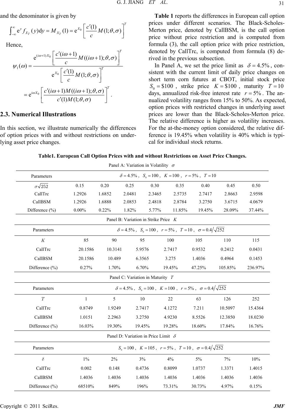








;).









G. J. JIANG ET AL.
31
and the denominator is given by
0(1)
e()d(1)e(1;,)
TT
T
X yXX
c
fyyM M
c












Hence,
0
0
(1)
1
(1)
e((1
()
(1)
e(1;,)
T
iX
T
X
ci Mi
c
cM
c













);,)



0(1)((1);,)
e.
(1)(1; ,)
T
iX ciM i
cM



  



2.3. Numerical Illustrations
In this section, we illustrate numerically the d
of option prices with and without restrictions on under-
Table 1 reports the differences in European call option
pr
mit as
ices under different scenarios. The Black-Scholes-
Merton price, denoted by CallBSM, is the call option
price without price restriction and is computed from
formula (3), the call option price with price restriction,
denoted by CallTrc, is computed from formula (8) de-
rived in the previous subsection.
In Panel A, we set the price li4.5%

,
ice chang
con-
sistent with the current limit of daily pres on
short term corn futures at CBOT, initial stock price
0$100S

, strike price $100K, maturity 10T

lized risk-free ine 5%r. T
nualized volatility ranges from 15% to 5 expected,
option prices with restricted changes in underlying asset
prices are lower than the Black-Scholes-Merton price.
The relative difference is higher as volatility increases.
For the at-the-money option considered, the relative dif-
ference is 19.45% when volatility is 40% which is typi-
cal for individual stock returns.
days, annuaterest rathe an-
ifferences
lying asset price changes.
0%. As
Table1. European Call Option Prices with and without Restrictions on Asset Prie Changes.
on in Volatility
c

Panel A: Variati
4.5%  ,
Parameters 0100S, 100K, 5%r, 10T

252s 0.15 0.20 0.25 0.30 0.35 0.40 0.45 0.50
CallTrc 1.2926 1.6822.7417 2.8663 2.9598
1.2926 1.6888 2.0853 2.4818 2.8784 3.6715 4.0679
Difference ) 0 1 1 2 3
52 2.0481 2.3465 .5735
CallBSM 3.2750
(%0.00%.22% 1.82% 5.77%1.85%9.45%8.09%7.44%
Panel Bn in ice: VariatioStrike Pr
K
Parameters , 100 , r, 1T
0
S, 4.5% 5%

00.4  252



85 90 95 100 105 110 115 K
CallTrc 20.1586 0.9532 0.2412 0.0431
20.1586 10.489 3565 3.275 0.0.1453
Difference (%) 0. 1. 6. 1 4 10 23
10.3141 5.9576 2.7417
CallBSM 6.1.4036 4964
27%70%70%9.45% 7.25%5.85%6.97%
Panel C: Variation in Maturit
Para
y T
meters 0100S, 100K,

, 5%4.5%


r

, 0.4 252  
T 1 5 63 126 252 10 22
CallTrc 0.8749 1.7.211 10.5097 15.4364
1.0151 2.2963 3.2750 4.9230 8.26 12.3850 18.0230
Difference (%) 16.% 19. 19 19 18. 1 1
9249 2.7417 4.1272
CallBSM 55
0330%.45%.28%60% 7.84%6.76%
Panel D: Variarice Lition in Pmit

Parameters 0100S, 105K

, 5%r

, 10T

, 0.4 252  
d 1% 5% 7% 10% 2% 3% 4%
CallTrc 0.002 0.148 0.4736 0.8099 1.0737 1.3371 1.4015
1.4036 1.4036 1.4036 1.4036 4036 1.1.4036
Difference (%) 68 849% 196% 7 3 4.
CallBSM 1.4036
510%3.31%0.73%97%0.15%

G. J. JIANG ET AL.
32
As expectedhe option srice isr, the
relative difference also increases. The results are illus-
trated in Panel B volatility is set as 40%
um and th ranges85 t. We
o
-money tions
y increases to 6-month () and 1-
ye
, when ttrike p highe
where per an-
n
n
e strike price from $o $115
te that when the strike price $110K, $115, the
relative differences are more than 100% and 200%, re-
spectively.
Panel C illustrates the differences in option prices with
different maturities. For the at-theop con-
sidered, the relative differences are rather consistent even
when maturit126T
ar (252T).
Panel D illustrates the effect of daily price limits on
option prices, where

is set to values in a range of 1%
to 10%. As expected, the relative differereases as
the abpric
nce inc
solute e t is lower. For the out-of-the-
m
o
changes often set daily limits for the price
hanges of traded assets. These restrictions have a dir
options traded on these assets
ey rt drahangasset. In this
aper,rive ormn of pricing
rmula with restrictions oninprice
hangng nal exs, weate that
i is supported by NSFC
61053).
. References
and M. Scholes, “The Pricing of Options and
Corporate Liabilities,” Journal of Political Economy, Vol.
, pp. 637-654. doi:10.1086/260062
limi
oney option considered (strike price 105K), the
relative difference inption price with restriction and
without restriction is more than 30% when the price limit
is set as 5%.
3. Conclusions
In practice, ex
cect
since impact on prices of
thule oumatic ces in prices
p
fo
we declosed-f solutio
underly
option
g asset
ces. Usiumericample illustr
very often the impact of such restrictions on option
prices can be substantial.
6. Acknowledgements
The research of Lei Sh
(111
5
[1] F. Black
81, No. 3, 1973
] R. C. Merton, “Theory of Rational Option Pricing,” Bell [2 Journal of Economics, Vol. 4, No. 1, 1973, pp. 141-183.
doi:10.2307/3003143
[3] J. C. Hull, “Options, Futures, and Other Derivatives,” 8th
ith Applications to Bond and Cur-
Edition, Prentice Hall, Upper Saddle River, 2011.
[4] S. L. Heston, “A Closed-Form Solution for Options with
Stochastic Volatility w
rency Options,” Review of Financial Studies, Vol. 6, No.
2, 1993, pp. 327-343. doi:10.1093/rfs/6.2.327

G. J. JIANG ET AL.
33
ppendix
the appendix, we first derive the moment generating
nction (mgf), and characteristic function (CF) of a
al random variable. Recall that the pdf of
truncated normal random variable )
A
In
fu
truncated norm
a2
trc
~(,X



,
trc
1
() ()
f
xfx
c
, [,]
x
ab



,
where ()
f
x is the normal density function and
1
ba
c

 
 
 
 . (10)
mgf able as
)
The of a truncated normal random vari
2
trc
~(,X



is derived as,
2
()
1
e e
x
bx2
2
2
22 2
trc trc
2
()
1
2 2
()ee ()d
d
2π
11
eed
2π
()
()
b
Xx
a
a
x
b
a
ME fxx
x
c
x
c
cM
c






 
























where





22
1
2
() eM




 is the mgf of a normal random
variable, and
2
2
2
2
() d
2
a
cx
22
22
22
()
() ()
22
22
1e
π
11
ed ed
2π2π
() ()
1.
x
b
xx
ba
x
x
ba
ba








 

 






 
 
 


 



  
 



  




Similarly, the characteristic function (CF) of a trun-
cated normal random variable )





2
trc
~(,X



is given
by,
trc trc
()
()( )()
ci
Mi c


 

 ,
where c is given by (10), and
22
1
2
() e
i




,
is the CF of a normal random variable,
() 1
b
i i 

a
ci 



 

 


.
Next, we derive the CF of the log price with truncated
distribution. Denote 1T
Z
XX


2
1trc
,,~(, )
T
XX as the sum of the iid sequence

 

, then the mgf of
Z
is

trc
()
(;,,,) ()( ,)
T
T
Zc
MabM M
c

 





Z
and the CF of is

trc
()
(;,,,) ()()
T
T
Zci
ab c







,
where we emphasize that the characteristic function
Z

eters also depends on normal random variable param
,

 and truncation parameters
Denote as the stock price at end of day
,ab.
the
t
S t and
ln
tt
X
S

,T
distribute
),
is the log price. Suppose we have trading
, and the daily log returns ar
d in a risk-neutral world,
T
i.e.
days, 1,
normally
2
(,
trc
e iid truncated
, ~
t
Y



1
(lnln,1,,
ttt
YSSt T
).


day T is
The log price
at the end of
0
1
T
Tt
t
X
XY



, 2
trc
~ iid(,)
t
Y



.
The mgf and CF of are derived as
T
X
0()
() ee()
T
T
T
X X
Xc
ME M
c
 







 
,
0()
() ee()
T
T
T
iX iX
Xci
Ec
 
 





 
,
where
1
ba
c

 


 
 ,
() 1
ba
c


 


  
 
 
,
22
1
2
() eM




, normal mgf
22
1
2
() e
i





, normal CF.